

Lee-Huang-Yang correction for bright soliton solutions of single and two component Bose-Einstein condensates
-
摘要: 李黄杨(LHY)修正是指玻色-爱因斯坦凝聚体中的自陷态,通过平均场(MF)态周围的量子涨落引起的有效自排斥来稳定,但LHY修正可能会影响玻色-爱因斯坦凝聚体亮孤子的基态,导致亮孤子试探解产生一定的适用范围。本研究利用变分近似法和以Gross-Pitaevskii方程为基础的数值模拟方法,通过将准一维情况单分量和二分量的玻色-爱因斯坦凝聚体基态模型加入LHY修正,计算了2个系统的试探解和数值模拟解。计算表明,对于准一维带有LHY项的单分量和二分量玻色-爱因斯坦凝聚体,当系统的LHY系数G在一定情况下可以通过变分法得到较好的静态近似解。本文的研究对于获得准一维情况下带有LHY项的单分量和二分量玻色-爱因斯坦凝聚体的基态解析解的条件提供了理论支持,为今后研究该系统的性质和物理内涵提供了帮助。
-
关键词:
- 玻色-爱因斯坦凝聚 /
- 自旋-轨道耦合 /
- 李黄杨(LHY)修正
Abstract: The Lee-Huang-Yang(LHY)correction refers to the self trapping state in the Bose Einstein condensates, which is stabilized through effective self repulsion caused by quantum fluctuations around the mean field(MF)state. However, the LHY correction may affect the ground state of bright solitons in Bose Einstein condensates, leading to a certain range of applicability for the experimental solution of bright solitons. This study utilized variational approximation and numerical simulation methods based on the Gross Pitaevskii equation. By incorporating LHY corrections to the ground state models of quasi one-dimensional Bose Einstein condensates with single and two components, the experimental and numerical simulation solutions of the two systems were calculated. The calculation shows that for quasi one-dimensional single component and two component Bose Einstein condensates with LHY terms, good static approximate solutions can be obtained through the variational method under certain conditions for the LHY coefficient G of the system. The research in this article provides theoretical support for obtaining the ground state analytical solutions of single and two component Bose Einstein condensates with LHY terms in the quasi one-dimensional case, and provides assistance for future research on the properties and physical connotations of the system. -
0. 引言
1925年,爱因斯坦预言当玻色子体系达到某一临界温度时,粒子就会大量聚集在某个低能量的模式,这种现象被称为玻色-爱因斯坦凝聚(Bose-Ein‐ stein condensation,BEC)[1-2]。BEC现象首次在1995年被观测到[3],其性质用Gross-Pitaevskii(GP)方程来描述。GP方程在非线性现象中具有应用,如非线性光学[4-7]、引力物理[8-11]、约瑟夫森效应[12-13]和凝聚态物理[14]。但GP方程的准确求解有一定困难,需要进行数值模拟来求解。
2011年首次实现中性原子的自旋- 轨道耦合[15],是研究量子现象的良好平台,如液氦中的超流动性[16]和金属中的超导性[17]。因为自旋-轨道耦合效应使单粒子基态简并,所以具有自旋-轨道耦合的旋量BEC表现出多种相和更丰富的基态相图[18-24]。旋量BEC的每个阶段都有自己的特点[25-28],如平面波相具有非零磁化强度,驻波相具有超固体特性[29],零动量相类似于没有自旋-轨道耦合的传统BEC。此外,自旋-轨道耦合效应导致了许多有趣的动态现象[30-35]。对于具有自旋-轨道耦合的BEC研究,Wen等[36]利用变分法导出了试探波函数的变分参数所满足的欧拉-拉格朗日方程,然后求解欧拉-拉格朗日方程的固定点解,提出了变分计算结果与GP方程数值模拟求得的基态解相吻合的区间。
1957年,杨振宁、李政道和黄克逊用赝势的办法导出了超越平均场理论,也就是李黄杨(LeeHuang-Yang,LHY)项[37]。LHY项是指BEC中的自陷态通过平均场(mean field,MF)态周围的量子涨落引起的有效自排斥来稳定[38]。LHY项可能会改变凝聚态的基态,如在强接触相互作用费米[39-41]和玻色气体[42-43]中观察到。LHY项提供了一个额外的排斥项,阻止了偶极坍缩,导致量子液滴的形成,这是一种新的物质状态[44-50]。Gangwar[51]提出了在有LHY项的情况下自束缚基态的结构和动力学的数值结果,但对于基态的研究还不充分且没有算试探解的适用范围。本文研究加上LHY项的单分量和二分量的BEC基态解和试探解的适用范围。
1. 单分量BEC亮孤子解的LHY修正
1.1 具有接触势的BEC亮孤子解
对于具有接触势的BEC,考虑沿x方向的准一维具有接触势的BEC,其能量表达式为
$$ \begin{gathered} E=\int_{-\infty}^{+\infty} \psi^*(x, t)\left(-\frac{\hbar^2}{2 m} \frac{\partial^2}{\partial x^2}+V(x)\right) \psi(x, t) \mathrm{d} x+ \\ \frac{1}{2} g \int_{-\infty}^{+\infty}|\psi(x, t)|^4 \mathrm{~d} x, \end{gathered} $$ (1) 式中:ψ (x) 是描述系统状态的波函数;V (x) 是系统所在的势阱;m是原子质量;$g=\frac{4 \pi \hbar^2 a_s}{m}$是相互作用系数(因为研究的是亮孤子动力学性质,其应在g < 0的情况存在);as是s波散射长度。系统的动力学性质可以由无量纲化的GP方程描述为
$$ \mathrm{i} \frac{\partial \psi}{\partial t}=\left(-\frac{1}{2} \frac{\partial^2}{\partial x^2}+V(x)\right) \psi+g|\psi|^2 \psi \text {, } $$ (2) 式中:ψ (x,t) 是描述动力学系统的波函数,满足归一化条件$\int_{-\infty}^{+\infty}|\psi(x, t)|^2 \mathrm{~d} x=1$;x和t分别是空间坐标和时间。在不考虑势阱的情况下,通过变分近似方法可以解析求得该体系下的动力学性质,体系的拉格朗日量为
$$ \begin{gathered} \mathcal{L}(t)= \\ \int_{-\infty}^{+\infty}\left[\frac{\mathrm{i}}{2}\left(\psi^* \frac{\partial \psi}{\partial t}-\psi \frac{\partial \psi^*}{\partial t}\right)+\frac{1}{2} \psi^* \frac{\partial^2 \psi}{\partial x^2}-\frac{g}{2}|\psi|^4\right] \mathrm{d} x 。 \end{gathered} $$ (3) 利用双曲函数作为亮孤子的试探波函数求该体系下的解析解,试探波函数为
$$ \psi(x, t)=\sqrt{\frac{\eta}{2}} \mathrm{e}^{\mathrm{i}(k x+\varphi)} \operatorname{sech}[\eta(x-\langle x\rangle)], $$ (4) 式中:η− 1为亮孤子的宽度;k为波矢;〈x〉是质心坐标;φ代表亮孤子试探解的相位,其都是时间的函数。将波函数代入到拉格朗日量中,可以得到
$$ \mathcal{L}(t)=-\langle x\rangle \frac{\mathrm{d} k}{\mathrm{~d} t}-\frac{\mathrm{d} \varphi}{\mathrm{d} t}-\frac{k^2}{2}-\frac{\eta^2}{6}-\frac{g \eta}{6} 。 $$ (5) 通过欧拉-拉格朗日方程$\frac{\partial \mathcal{L}}{\partial A}-\frac{\mathrm{d}}{\mathrm{d} t}\left(\frac{\partial \mathcal{L}}{\partial \dot{A}}\right)=0$,其中A是变分参数η、k、〈x〉和φ,并且$\dot{A}=\frac{\mathrm{d} A}{\mathrm{~d} t}$,代入可得变分参数随时间演化的运动方程为:
$$ \eta=-\frac{g}{2} $$ (6a) $$ \frac{\mathrm{d}\langle x\rangle}{\mathrm{d} t}=k, $$ (6b) $$ \frac{\mathrm{d} k}{\mathrm{~d} t}=0 \text { 。 } $$ (6c) 通过令$\frac{\mathrm{d}\langle x\rangle}{\mathrm{d} t}=0$,可以求得欧拉-拉格朗日方程的固定点解,由于〈x〉和k为常数,本文考虑其等于0的情况,取φ = 0,固定点解则为ψ = $\sqrt{\frac{-g}{4}} \operatorname{sech}\left[-\frac{g}{2} x\right]$。
由于变分法是一种近似方法,因此可以将其与GP方程的数值解作对比。数值求解基态方程的本质是虚时演化,本文采用了Crank-Nicolson方法进行数值模拟得到基态解,无量纲化后采用的势阱是谐振子势$V(x)=\frac{1}{2} x^2$,为了便于调节势阱的大小,将势阱改为$V(x)=\frac{1}{2} \lambda^2 x^2$,其中λ为势阱调节因子。计算结果如图 1所示,其中参数g =− 10,λ = 2。由图可知,欧拉-拉格朗日方程得到的变分亮孤子试探解与GP方程数值模拟得到的数值解相符,因此在具有接触势的BEC系统下,变分法可以得到一个比较好的基态解。
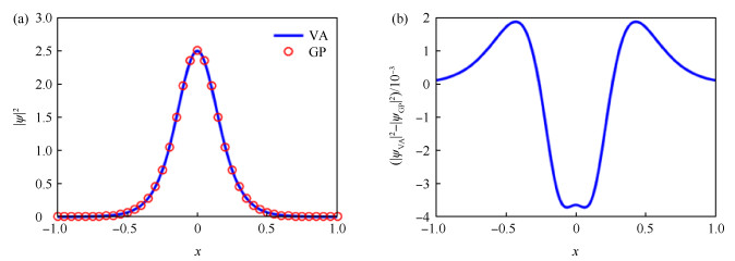 图 1 具有接触势的玻色-爱因斯坦凝聚体(BEC)试探解与数值解比较注:VA表示变分法的试探解;GP表示数值解。
(a)具有接触势的BEC变分试探解与数值解对比;(b)具有接触势的BEC变分试探解与数值解的差 下载:
全尺寸图片
1.2 具有接触势的BEC亮孤子解的LHY修正
对于带有LHY项的具有接触势的BEC,考虑沿x方向的带有LHY项的准一维具有接触势的BEC,其能量表达式为
$$ \begin{aligned} E= & \int_{-\infty}^{+\infty}{ }_\psi \psi^*(x, t)\left(-\frac{\hbar^2}{2 m} \frac{\partial^2}{\partial x^2}+V(x)\right) \psi(x, t) \mathrm{d} x+ \\ & \frac{1}{2} g \int_{-\infty}^{+\infty}|\psi(x, t)|^4 \mathrm{~d} x-\int_{-\infty}^{+\infty} G|\psi(x, t)|^3 \mathrm{~d} x, \end{aligned} $$ (7) 式中G是LHY项的作用系数。系统的动力学性质可以由无量纲化的GP方程描述为
$$ \mathrm{i} \frac{\partial \psi}{\partial t}=\left(-\frac{1}{2} \frac{\partial^2}{\partial x^2}+V(x)\right) \psi+g|\psi|^2 \psi-\frac{3}{2} G|\psi| \psi_{\circ} $$ (8) 在不考虑势阱的情况下,可以通过变分近似方法解析求得该系统的动力学性质,体系的拉格朗日量为
$$ \begin{gathered} \mathcal{L}(t)= \\ \int_{-\infty}^{+\infty}\left[\frac{i}{2}\left(\psi^* \frac{\partial \psi}{\partial t}-\psi^* \frac{\partial \psi^*}{\partial t}\right)+\frac{1}{2} \psi^* \frac{\partial^2 \psi}{\partial x^2}-\frac{g}{2}|\psi|^4+G|\psi|^3\right] \mathrm{d} x 。 \end{gathered} $$ (9) 利用双曲函数作为亮孤子的试探波函数求该体系下的解析解,试探波函数为
$$ \psi(x, t)=\sqrt{\frac{\eta}{2}} \mathrm{e}^{\mathrm{i}(k x+\varphi)} \operatorname{sech}[\eta(x-\langle x\rangle)] 。 $$ (10) 将波函数代入到拉格朗日量中,可以得到
$$ \mathcal{L}(t)=-\langle x\rangle \frac{\mathrm{d} k}{\mathrm{~d} t}-\frac{\mathrm{d} \varphi}{\mathrm{d} t}-\frac{k^2}{2}-\frac{\eta^2}{6}-\frac{g \eta}{6}+\frac{\sqrt{2 \eta}}{8} G \pi 。 $$ (11) 通过欧拉-拉格朗日方程$\frac{\partial \mathcal{L}}{\partial A}-\frac{\mathrm{d}}{\mathrm{d} t}\left(\frac{\partial \mathcal{L}}{\partial \dot{A}}\right)=0$,其中A是变分参数η、k、〈x〉和φ,并且$\dot{A}=\frac{\mathrm{d} A}{\mathrm{~d} t}$,代入可得变分参数随时间演化的运动方程为:
$$ -\frac{\eta}{3}-\frac{g}{6}+\frac{\sqrt{2}}{16 \sqrt{\eta}} G \pi=0 $$ (12a) $$ \frac{\mathrm{d}\langle x\rangle}{\mathrm{d} t}=k, $$ (12b) $$ \frac{\mathrm{d} k}{\mathrm{~d} t}=0 \text { 。 } $$ (12c) 通过令$\frac{\mathrm{d}\langle x\rangle}{\mathrm{d} t}=0$,可以求得欧拉-拉格朗日的固定点解,取〈x〉,k和φ为0,固定点解则为$\psi=\sqrt{\frac{\eta}{2}} \operatorname{sech}[\eta x]$。由于η满足的方程(12a)是一元三次方程,需要运用卡尔达诺公式求解并在判别式的不同条件下讨论根的性质,选择符合条件的固定点解。将其与GP方程的数值解作对比,采用Crank-Nicolson方法进行数值模拟,采用无量纲化的谐振子势阱V (x) = $\frac{1}{2} \lambda^2 x^2$。通过实验表明,加入LHY项后,当LHY系数$(G) \geqslant-\sqrt{\frac{-64}{243 \pi^2} g^3}$时,系统通过欧拉-拉格朗日方程所得到的变分亮孤子试探解可以与GP方程模拟出的数值解相符,所以针对加入LHY项的具有接触势的准一维BEC,G在上述取值范围时依然可以得到较好的基态解,结果如图 2所示,分图中参数分别为(a)g =− 10,λ = 0.01,G =− 5;(b)g =− 10,λ = 0.01,G =− 1;(c)g =− 10,λ = 0.01,G = 5;(d)g = − 10,λ= 0.01,G =− 5;(e)g =− 10,λ= 0.01,G =− 1;(f)g =− 10,λ = 0.01,G = 5。
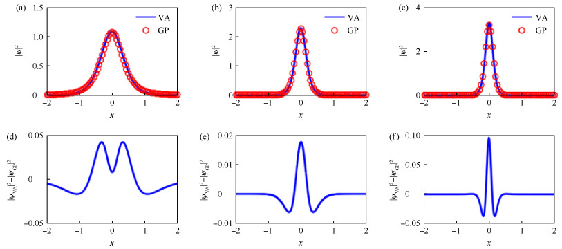 图 2 不同李黄杨(LHY)系数(G)下具有接触势的BEC变分试探解与数值解比较(a~c)表示G=−5、-1和5时具有接触势的BEC变分试探解与数值解对比;(d~f) 表示G=−5、-1和5时具有接触势的BEC变分试探解与数值解的差下载:
全尺寸图片
当$G<-\sqrt{\frac{-64}{243 \pi^2} g^3}$时,通过数值求根显示并没有符合条件的η值,从而没有符合条件的变分亮孤子试探解。因此,G在上述取值范围时的亮弧子固定点解不可用。
2. 二分量BEC亮孤子解的LHY修正
2.1 具有自旋-轨道耦合的BEC亮孤子解
对于具有自旋-轨道耦合的BEC,考虑沿x方向的准一维具有自旋-轨道耦合的二分量BEC,其能量表达式为
$$ \begin{aligned} E= & \int_{-\infty}^{+\infty}\left[\left(\psi_i^*(x, t), \psi_{\downarrow}^*(x, t)\right)\left(\frac{\left(\hat{p}_x+\hbar k_r \sigma_z\right)^2}{2 m}+\frac{\delta_a}{2} \sigma_z+\frac{\Omega}{2} \sigma_x+V(x)\right)\binom{\psi_{+}(x, t)}{\psi_{\downarrow}(x, t)}\right] \mathrm{d} x+ \\ & \frac{1}{2} \int_{-\infty}^{+\infty}\left[\left(2 g_{\dagger \downarrow}\left|\psi_{\uparrow}(x, t)\right|^2\left|\psi_{\downarrow}(x, t)\right|^2+g_{\dagger \dagger}\left|\psi_{\uparrow}(x, t)\right|^4+g_{+4}\left|\psi_{\downarrow}(x, t)\right|^4\right] \mathrm{d} x, \right. \end{aligned} $$ (13) 式中:$\psi_s(x, t)(s=\uparrow, \downarrow \text {, 代表 } 2 \text { 个不同的组分 })$是描述系统状态的波函数;σ x 和σz代表泡利矩阵;V (x) 是系统所在的势阱;$\hat{p}_x$是动量算符;kr是激光的波矢;Ω是拉曼耦合强度;δa是失谐量;g↑↑和g↓↓是种内原子相互作用强度;g↑↓是种间原子相互作用强度。
考虑沿x方向的准一维具有自旋-轨道耦合的二分量BEC,由于二分量的g↑↑、g↓↓和g↑↓接近,假设三者相等,在不考虑势阱的情况下,系统的动力学性质可以由无量纲化的GP方程描述[36]:
$$ \mathrm{i} \frac{\partial \psi_{\uparrow}}{\partial t}=-\frac{1}{2} \frac{\partial^2 \psi_{\uparrow}}{\partial x^2}-\mathrm{i} k_r \frac{\partial \psi_{\uparrow}}{\partial x}+\frac{\delta_a}{2} \psi_{+}+\frac{\Omega}{2} \psi_{+}+g n \psi_{\uparrow}, $$ (14) $$ \mathrm{i} \frac{\partial \psi_{\downarrow}}{\partial t}=-\frac{1}{2} \frac{\partial^2 \psi_{+}}{\partial x^2}+\mathrm{i} k_r \frac{\partial \psi_{+}}{\partial x}-\frac{\delta_a}{2} \psi_{+}+\frac{\Omega}{2} \psi_{\uparrow}+g n \psi_{\downarrow} 。 $$ (15) 式中:ψ s (x,t) 是描述二分量动力学系统的波函数,其满足归一化$\sum\limits_{s=\uparrow, \downarrow} \int_{-\infty}^{+\infty}\left|\psi_s(x, t)\right|^2 \mathrm{~d} x=1 ; n=\left|\psi_{\uparrow}\right|^2+\left|\psi_{\downarrow}\right|^2 $代表了总密度分布。通过变分近似方法可以解析求得系统的动力学性质,体系的拉格朗日量为[36]
$$ \mathcal{L}(t)=\int_{-\infty}^{+\infty}\left[\begin{array}{c} \frac{\mathrm{i}}{2} \sum\limits_{s=\uparrow, \downarrow}\left(\psi_s^* \frac{\partial \psi_s}{\partial t}-\psi_s \frac{\partial \psi_s^*}{\partial t}\right)+\frac{1}{2} \psi_{\uparrow}^* \frac{\partial^2 \psi_{\uparrow}}{\partial x^2}+\frac{1}{2} \psi_{!}^* \frac{\partial^2 \psi_{\downarrow}}{\partial x^2}+\mathrm{i} k_r\left(\psi_{\uparrow}^* \frac{\partial \psi_{\uparrow}}{\partial x}-\psi_{!}^* \frac{\partial \psi_{\downarrow}}{\partial x}\right)- \\ \frac{\delta_a}{2}\left(\left|\psi_{\uparrow}\right|^2-\left|\psi_{\downarrow}\right|^2\right)-\frac{\Omega}{2}\left(\psi_{\uparrow}^* \psi_{\downarrow}+\psi_{\dagger}^* \psi_{\uparrow}\right)-\frac{g}{2} n^2 \end{array}\right] \mathrm{d} x_0 $$ (16) 文献[36]中利用双曲函数作为亮孤子的试探波函数求该体系下的解析解,试探波函数为[36]
$$ \binom{\psi_{\uparrow}(x, t)}{\psi_{\downarrow}(x, t)}=\sqrt{\frac{\eta}{2}}\binom{\sin \theta \mathrm{e}^{\mathrm{i}\left(k x+\varphi_{\uparrow}\right)}}{\cos \theta \mathrm{e}^{\mathrm{i}\left(k x+\varphi_{\downarrow}\right)}} \operatorname{sech}[\eta(x-\langle x\rangle)], $$ (17) 式中:φs代表二分量试探解的相位;θ用来描述二分量试探解的振幅比,其他都是时间的函数。将波函数代入到拉格朗日量中,定义$\varphi_{ \pm}=\frac{\varphi_{\uparrow} \pm \varphi_{\downarrow}}{2}, \beta=k_r k+\frac{\delta_a}{2}$,可以得到[36]
$$ \begin{gathered} \mathcal{L}(t)=-\langle x\rangle \frac{\mathrm{d} k}{\mathrm{~d} t}+\cos (2 \theta) \frac{\mathrm{d} \varphi_{-}}{\mathrm{d} t}-\frac{\mathrm{d} \varphi_{+}}{\mathrm{d} t}+\beta \cos (2 \theta)- \\ \frac{\Omega}{2} \sin (2 \theta) \cos \left(2 \varphi_{-}\right)-\frac{\eta(\eta+g)}{6}-\frac{1}{2} k^2 \end{gathered} $$ (18) 通过欧拉-拉格朗日方程$\frac{\partial \mathcal{L}}{\partial A}-\frac{\mathrm{d}}{\mathrm{d} t}\left(\frac{\partial \mathcal{L}}{\partial \dot{A}}\right)=0$,其中A是变分参数η、k、〈x〉、φ±和θ,并且$\dot{A}=\frac{\mathrm{d} A}{\mathrm{~d} t}$,代入可得变分参数随时间演化的运动方程[36]:
$$ \eta=-\frac{g}{2} $$ (19a) $$ \frac{\mathrm{d} k}{\mathrm{~d} t}=0 $$ (19b) $$ \frac{\mathrm{d}\langle x\rangle}{\mathrm{d} t}=k-k_r \cos (2 \theta), $$ (19c) $$ \frac{\mathrm{d} \theta}{\mathrm{d} t}=-\frac{\Omega}{2} \sin \left(2 \varphi_{-}\right), $$ (19d) $$ \frac{\mathrm{d} \varphi_{-}}{\mathrm{d} t}=-\beta-\frac{\Omega}{2} \cot (2 \theta) \cos \left(2 \varphi_{-}\right) \text {。 } $$ (19e) 通过令$\frac{\mathrm{d}\langle x\rangle}{\mathrm{d} t}=\frac{\mathrm{d} \varphi_{-}}{\mathrm{d} t}=\frac{\mathrm{d} \theta}{\mathrm{d} t}=0$,可以求得欧拉-拉格朗日方程的固定点解,将固定点解中的符号用“~”标记。此时〈x〉为任意的常数,$\varphi_{-}=n \frac{\pi}{2}$,其中n为整数。θ͂和k͂的解满足方程组[36]:
$$ \tilde{k}-k_r \cos (2 \tilde{\theta})=0 \text {, } $$ (20a) $$ k_r{ }^2 \cos (2 \tilde{\theta})+\frac{\delta_a}{2}+\frac{\Omega}{2} \cot (2 \tilde{\theta}) \cos \left(2 \varphi_{-}\right)=0 \text { 。 } $$ (20b) 考虑了n = 0、〈x〉= 0的情况。取φ− = 0,将变分亮孤子试探解与GP方程的数值模拟解进行对比,使用Crank-Nicolson方法,采用无量纲化的谐振子势阱$V(x)=\frac{1}{2} \lambda^2 x^2$。结果如 图 3所示,其中:(a)kr = 0.10;(b)kr = 0.75,其他参数为δa = 0.6,Ω = 1,g =− 10。
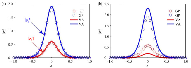 图 3 不同kr下变分试探解与GP方程数值解的对比注:蓝色线代表自旋向下波函数(|ψ↓2 |);红色线代表自旋向上波函数(|ψ↓2 |)。
(a)弱自旋-轨道耦合下变分试探解与数值解对比;(b)强自旋-轨道耦合下变分试探解与数值解对比下载:
全尺寸图片
文献[36]结果显示:对于弱自旋-轨道耦合的情况$\left(\frac{\Omega}{k_r{ }^2} \gg 1\right)$,欧拉-拉格朗日方程的变分亮孤子试探解与GP方程的数值解相一致;对于强自旋-轨道耦合的情况$\left(\frac{\Omega}{k_r^2} \ll 1\right)$,二者则有差别。
2.2 具有自旋-轨道耦合的BEC亮孤子解的LHY修正
对于本文所研究带有LHY项的具有自旋-轨道耦合的BEC,考虑沿x方向的准一维情况,其能量表达式为
$$ \begin{aligned} & E=\int_{-\infty}^{+\infty}\left[\begin{array}{c} \left(\psi_{\uparrow}^*(x, t), \psi_{\downarrow}^*(x, t)\right)\left(\frac{\left(\hat{p}_x+\hbar k_r \sigma_z\right)^2}{2 m}+\right. \\ \left.\frac{\delta_a}{2} \sigma_z+\frac{\Omega}{2} \sigma_x+V(x, t)\right)\left(\begin{array}{l} \psi_{\uparrow}(x, t) \\ \psi_{\downarrow}(x, t) \end{array}\right] \end{array}\right] \mathrm{d} x+ \\ & \frac{1}{2} \int_{-\infty}^{+\infty}\left[\left(2 g_{\uparrow \downarrow}\left|\psi_{\uparrow}(x, t)\right|^2\left|\psi_{\downarrow}(x, t)\right|^2+g_{\uparrow \uparrow}\left|\psi_{\uparrow}(x, t)\right|^4+\right.\right. \\ & \left.g_{\downarrow \downarrow}\left|\psi_{\downarrow}(x, t)\right|^4 \mathrm{~d} x\right]-\int_{-\infty}^{+\infty} G n^{\frac{3}{2}} \mathrm{~d} x 。 \\ & \end{aligned} $$ (21) 在不考虑势阱的情况下,系统的动力学性质可以由无量纲化的GP方程描述:
$$ \begin{gathered} \mathrm{i} \frac{\partial \psi_{\uparrow}}{\partial t}=-\frac{1}{2} \frac{\partial^2 \psi_{\uparrow}}{\partial x^2}-\mathrm{i} k_r \frac{\partial \psi_{\uparrow}}{\partial x}+\frac{\delta_a}{2} \psi_{\uparrow}+\frac{\Omega}{2} \psi_{\downarrow}+ \\ g n \psi_{\uparrow}-\frac{3}{2} G \sqrt{\left|\psi_{\uparrow}\right|^2+\left|\psi_{\downarrow}\right|^2} \psi_{\uparrow}, \end{gathered} $$ (22) $$ \begin{gathered} \mathrm{i} \frac{\partial \psi_{\downarrow}}{\partial t}=-\frac{1}{2} \frac{\partial^2 \psi_{\downarrow}}{\partial x^2}+\mathrm{i} k_r \frac{\partial \psi_{\downarrow}}{\partial x}-\frac{\delta_a}{2} \psi_{\downarrow}+\frac{\Omega}{2} \psi_{\uparrow}+ \\ g n \psi_{\downarrow}-\frac{3}{2} G \sqrt{\left|\psi_{\uparrow}\right|^2+\left|\psi_{\downarrow}\right|^2} \psi_{\downarrow} \end{gathered} $$ (23) 通过变分近似方法可以解析求得系统的动力学性质,体系的拉格朗日量为
$$ \begin{aligned} &\quad \quad \quad \quad \quad \quad \quad \quad \quad \quad \mathcal{L}(t)= \\ & \int_{-\infty}^{+\infty}\left[\begin{array}{c} \frac{\mathrm{i}}{2} \sum\limits_{s=\uparrow,\downarrow}\left(\psi_s^* \frac{\partial \psi_s}{\partial t}-\psi_s \frac{\partial \psi_s^*}{\partial t}\right)+\frac{1}{2} \psi_{\uparrow}^* \frac{\partial^2 \psi_{\uparrow}}{\partial x^2}+ \\ \frac{1}{2} \psi_{\downarrow}^* \frac{\partial^2 \psi_{\downarrow}}{\partial x^2}+\mathrm{i} k_r\left(\psi_{\uparrow}^* \frac{\partial \psi_{\uparrow}}{\partial z}-\psi_{\downarrow}^* \frac{\partial \psi_{\downarrow}}{\partial z}\right)- \\ \frac{\delta_g}{2}\left(\left|\psi_{\uparrow}\right|^2-\left|\psi_{\downarrow}\right|^2\right)-\frac{\Omega}{2}\left(\psi_{\uparrow}^* \psi_{\downarrow}+\psi_{\downarrow}^* \psi_{\uparrow}\right)- \\ \frac{g}{2} n^2+G\left(\left|\psi_{\uparrow}\right|^2+\left|\psi_{\downarrow}\right|^2\right)^{\frac{3}{2}} \end{array}\right] \mathrm{d} x_{\circ} \\ & \end{aligned} $$ (24) 利用双曲函数作为亮孤子试探波函数求该体系下的解析解,试探波函数为
$$ \binom{\psi_{\uparrow}(x, t)}{\psi_{\downarrow}(x, t)}=\sqrt{\frac{\eta}{2}}\binom{\sin \theta \mathrm{e}^{\mathrm{i}\left(k x+\varphi_{\uparrow}\right)}}{\cos \theta \mathrm{e}^{\mathrm{i}\left(k x+\varphi_{\downarrow}\right)}} \operatorname{sech}[\eta(x-\langle x\rangle)], $$ (25) 将波函数代入到拉格朗日量中,定义$\varphi_{ \pm}=\frac{\varphi_{\uparrow} \pm \varphi_{\downarrow}}{2},\beta=k_r k+\frac{\delta_a}{2}$,可以得到
$$ \begin{gathered} \mathcal{L}(t)=-\langle x\rangle \frac{\mathrm{d} k}{\mathrm{~d} t}+\cos (2 \theta) \frac{\mathrm{d} \varphi_{-}}{\mathrm{d} t}-\frac{\mathrm{d} \varphi_{+}}{\mathrm{d} t}+\beta \cos (2 \theta)- \\ \frac{\Omega}{2} \sin (2 \theta) \cos \left(2 \varphi_{-}\right)- \\ \frac{\eta(\eta+g)}{6}-\frac{1}{2} k^2+G \pi \frac{\sqrt{2 \eta}}{8} . \end{gathered} $$ (26) 通过欧拉-拉格朗日方程$\frac{\partial \mathcal{L}}{\partial A}-\frac{\mathrm{d}}{\mathrm{d} t}\left(\frac{\partial \mathcal{L}}{\partial \dot{A}}\right)=0$,其中A是变分参数η、k、〈x〉、φ±和θ,并且$\dot{A}=\frac{\mathrm{d} A}{\mathrm{~d} t}$,代入可得变分参数随时间演化的运动方程:
$$ -\frac{\eta}{3}-\frac{g}{6}+\frac{\sqrt{2}}{16 \sqrt{\eta}} G \pi=0 \text {, } $$ (27a) $$ \frac{\mathrm{d} k}{\mathrm{~d} t}=0, $$ (27b) $$ \frac{\mathrm{d}\langle x\rangle}{\mathrm{d} t}=k-k_r \cos (2 \theta), $$ (27c) $$ \frac{\mathrm{d} \theta}{\mathrm{d} t}=-\frac{\Omega}{2} \sin \left(2 \varphi_{-}\right), $$ (27d) $$ \frac{\mathrm{d} \varphi_{-}}{\mathrm{d} t}=-\beta-\frac{\Omega}{2} \cot (2 \theta) \cos \left(2 \varphi_{-}\right) \text {。 } $$ (27e) 通过令$\frac{\mathrm{d}\langle x\rangle}{\mathrm{d} t}=\frac{\mathrm{d} \varphi_{-}}{\mathrm{d} t}=\frac{\mathrm{d} \theta}{\mathrm{d} t}=0$,可以求得欧拉- 拉格朗日方程的固定点解,同样将固定点解中的符号用“~”标记,显示固定点解中的$\tilde{\theta} \text { 和 } \tilde{k}$所满足的方程组与式(20a)和(20b)所研究的情况相同,不同点在于ῆ的取定满足方程(27a),采用卡尔达诺公式求解方程并选择合适的固定点解进行取舍。取φ− = 0,将亮孤子的固定点解与GP方程的数值解进行对比,数值模拟采用Crank-Nicolson方法,采用无量纲化的谐振子势阱$V(x)=\frac{1}{2} \lambda^2 x^2$。在弱自旋-轨道耦合的情况$\left(\frac{\Omega}{k_r{ }^2} \gg 1\right)$,选取不同的G结果如图 4所示,其他参数δa = 0.6,Ω = 1,g =− 10,kr = 0.1。
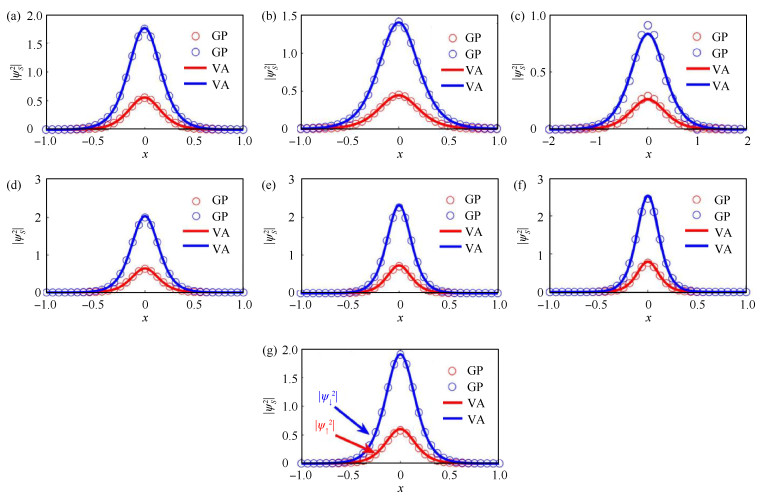 图 4 弱自旋-轨道耦合下不同G的试探解与数值解对比(a)G =− 1;(b)G =− 3;(c)G =− 5;(d)G = 1;(e)G = 3;(f)G = 5;(g)G = 0下载:
全尺寸图片
实验显示,在弱自旋-轨道耦合情况下,当G ≥ $-\sqrt{\frac{-64}{243 \pi^2} g^3}$时,在较弱的LHY项取值下,系统的亮孤子试探解与数值解相一致,随着G逐渐变强时,亮孤子试探解与数值解开始存在一定的偏差。
在强自旋-轨道耦合的情况$\left(\frac{\Omega}{k_r^2} \gg 1\right)$,选取不同的G结果如图 5所示,其他参数δa = 0.6,Ω = 1,g =− 10,kr = 0.75。
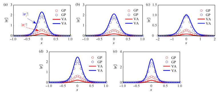 图 5 强自旋-轨道耦合下不同G的试探解与数值解对比(a)G = 0;(b)G =− 1;(c)G =− 5;(d)G = 1;(e)G = 5下载:
全尺寸图片
实验表明,在强自旋-轨道耦合情况下,当G ≥ $-\sqrt{\frac{-64}{243 \pi^2} g^3}$时,不同的LHY项取值下系统的亮孤子试探解与数值解并不一致;当G < $-\sqrt{\frac{-64}{243 \pi^2} g^3}$,由于在求根时并不存在符合条件的η解,因此在上述取值范围则无法找到合适的亮孤子试探解。
3. 结论
对于准一维带有LHY项的具有接触势的单分量BEC,当系统的G ≥ $-\sqrt{\frac{-64}{243 \pi^2} g^3}$时,系统通过欧拉-拉格朗日方程得到的亮孤子试探解可以与GP方程模拟出的数值解相符,所以变分法在上述情况可以得到一个很好的静态近似解。当系统的G < $-\sqrt{\frac{-64}{243 \pi^2} g^3}$时,通过数值求根显示并没有符合条件的η值,因此G在上述取值范围时亮孤子试探解不可用,则此时变分法所得静态近似解不可用。
对于准一维带有LHY项的具有自旋-轨道耦合的二分量BEC,在弱自旋-轨道耦合情况下,当G ≥ $-\sqrt{\frac{-64}{243 \pi^2} g^3}$时,系统选择较弱的LHY项取值时,亮孤子试探解与数值解相一致,此时变分法所得静态近似解较好。随着G逐渐变强时,亮孤子试探解与数值解开始存在一定的偏差,此时的变分法所得静态近似解不可用。而在强自旋-轨道耦合情况下,无论G取何值,变分法都无法得到合适的静态近似解。本研究对于获得带有LHY项的单分量和二分量BEC的基态解析解的条件提供了理论支持,为今后研究该系统的性质和物理内涵提供了帮助。
-
图 1 具有接触势的玻色-爱因斯坦凝聚体(BEC)试探解与数值解比较
注:VA表示变分法的试探解;GP表示数值解。
(a)具有接触势的BEC变分试探解与数值解对比;(b)具有接触势的BEC变分试探解与数值解的差下载:
全尺寸图片
图 2 不同李黄杨(LHY)系数(G)下具有接触势的BEC变分试探解与数值解比较
(a~c)表示G=−5、-1和5时具有接触势的BEC变分试探解与数值解对比;(d~f) 表示G=−5、-1和5时具有接触势的BEC变分试探解与数值解的差
下载:
全尺寸图片
图 3 不同kr下变分试探解与GP方程数值解的对比
注:蓝色线代表自旋向下波函数(|ψ↓2 |);红色线代表自旋向上波函数(|ψ↓2 |)。
(a)弱自旋-轨道耦合下变分试探解与数值解对比;(b)强自旋-轨道耦合下变分试探解与数值解对比下载:
全尺寸图片
图 4 弱自旋-轨道耦合下不同G的试探解与数值解对比
(a)G =− 1;(b)G =− 3;(c)G =− 5;(d)G = 1;(e)G = 3;(f)G = 5;(g)G = 0
下载:
全尺寸图片
图 5 强自旋-轨道耦合下不同G的试探解与数值解对比
(a)G = 0;(b)G =− 1;(c)G =− 5;(d)G = 1;(e)G = 5
下载:
全尺寸图片
-
[1] BOSE S N. Plancks gesetz und lichtquantenhypothese [J]. Zeitschrift für Physik, 1924, 26(1): 178-181. doi: 10.1007/BF01327326 [2] PETHICK C J, SMITH H. Bose-Einstein condensation in dilute gases[M]. Cambridge: Cambridge University Press, 2008. [3] ANDERSON M H, ENSHER J R, MATTHEWS M R, et al. Observation of Bose-Einstein condensation in a dilute atomic vapor[J]. Science, 1995, 269(5221): 198-201. doi: 10.1126/science.269.5221.198 [4] LIU W M, KENGNE E. Schrödinger equations in nonlinear systems[M]. Singapore: Springer, 2019. [5] EFREMIDIS N K, SIVILOGLOU G A, CHRISTODOULIDES D N. Exact X-wave solutions of the hyperbolic nonlinear Schrödinger equation with a supporting potential[J]. Physics Letters A, 2009, 373 (44): 4073-4076. doi: 10.1016/j.physleta.2009.09.008 [6] BARASHENKOV I V, ZEZYULIN D A, KONOTOP V V. Exactly solvable Wadati potentials in the PTsymmetric Gross-Pitaevskii equation[C]// BAGARELLO F, PASSANTE R. Non-Hermitian Hamiltonians in Quantum Physics: Selected Contributions from the 15th International Conference on NonHermitian Hamiltonians in Quantum Physics. Palermo, Italy: Springer International Publishing, 2016. [7] KIVSHAR Y S, AGRAWAL G P. Optical solitons: from fibers to photonic crystals[M]. London: Academic Press, 2003. [8] MOFFAT J W. Spectrum of cosmic microwave fluctuations and the formation of galaxies in a modified gravity theory[EB/OL]. (2006-2-27)[2023-8-10]. arXiv: astro-ph/0602607vl. [9] CUNILLERA F, GERMANI C. The Gross-Pitaevskii equations of a static and spherically symmetric condensate of gravitons[J]. Classical and Quantum Gravity, 2018, 35(10): 105006. doi: 10.1088/1361-6382/aab97b [10] YANG Y, WANG Y, ZHAO L, et al. Sonic black hole horizon formation for Bose-Einstein condensates with higher-order nonlinear effects[J]. AIP Advances, 2019, 9 (11): 115203. doi: 10.1063/1.5124934 [11] LEWANDOWSKY S, BALLARD T, PANCOST R D. Uncertainty as knowledge[J]. Philosophical Transactions of the Royal Society A(Mathematical, Physical and Engineering Sciences), 2015, 373 (2055): 0462. [12] ANGLIN J R, KETTERLE W. Bose-Einstein condensation of atomic gases[J]. Nature, 2002, 416 (6877): 211. doi: 10.1038/416211a [13] BURCHIANTI A, FORT C, MODUGNO M. Josephson plasma oscillations and the Gross-Pitaevskii equation: Bogoliubov approach versus two-mode model[J]. Physical Review A, 2017, 95(2): 023627. doi: 10.1103/PhysRevA.95.023627 [14] HAN J H. Skyrmions in condensed matter[M]. Berlin: Springer, 2017. [15] LIN Y J, JIMÉNEZ-GARCÍA K, SPIELMAN B I. Spinorbit-coupled Bose-Einstein condensates[J]. Nature, 2011, 471(7336): 83-86. doi: 10.1038/nature09887 [16] LEGGETT A J. Superfluidity[J]. Reviews of Modern Physics, 1999, 71: S318. doi: 10.1103/RevModPhys.71.S318 [17] CHEN Q J, STAJICB J, TAN S, et al. BCS-BEC crossover: from high temperature superconductors to ultracold superfluids[J]. Physics Reports, 2005, 412: 1-88. doi: 10.1016/j.physrep.2005.02.005 [18] WANG C J, GAO C, JIAN C M, et al. Spin-orbit coupled spinor Bose Einstein condensates[J]. Physical Review Letters, 2010, 105: 160403. doi: 10.1103/PhysRevLett.105.160403 [19] HO T L, ZHANG S Z. Bose-Einstein condensates with spin-orbit interaction[J]. Physical Review Letters, 2011, 107(15): 150403. doi: 10.1103/PhysRevLett.107.150403 [20] WEN L, SUN Q, WANG H Q, et al. Ground state of spin-1 Bose Einstein condensates with spin-orbit coupling in a Zeeman field[J]. Physical Review A, 2012, 86(4): 043602. doi: 10.1103/PhysRevA.86.043602 [21] LAN Z H, ÖHBERG P. The Raman-dressed spin-1 spinorbit-coupled quantum gas[J]. Physical Review A, 2013, 89(2): 023630. [22] NATU S S, LI X P, COLE W S. Striped ferronematic ground states in a spin-orbit-coupled S = 1 Bose gas[J]. Physical Review A, 2015, 91(2): 023608. doi: 10.1103/PhysRevA.91.023608 [23] SUN K, QU C L, XU Y, et al. Interacting spin-orbit coupled spin-1 Bose-Einstein condensates[J]. Physical Review A, 2016, 93(2): 023615. doi: 10.1103/PhysRevA.93.023615 [24] CAMPBELL D L, PRICE R M, PUTRA A, et al. Magnetic phases of spin-1 spin-orbit-coupled Bose gases [J]. Nature Communications, 2016, 7: 10897. doi: 10.1038/ncomms10897 [25] LI Y, PITAEVSKⅡ L P, STRINGARI S. Quantum tricriticality and phase transitions in spin-orbit coupled Bose-Einstein condensates[J]. Physical Review Letters, 2012, 108(22): 225301. doi: 10.1103/PhysRevLett.108.225301 [26] CHEN L, PU H, ZHANG Y B. Spin-orbit angular momentum coupling in a spin-1 Bose-Einstein condensate[J]. Physical Review A, 2016, 93(1): 013629. doi: 10.1103/PhysRevA.93.013629 [27] MÆLAND K, JANSSØNN A T G, RYGH J H, et al. Plane- and stripe-wave phases of a spin-orbit-coupled Bose-Einstein condensate in an optical lattice with a Zeeman field[J]. Physical Review A, 2020, 102(5): 053318. doi: 10.1103/PhysRevA.102.053318 [28] CHEN Y Y, LYU H, XU Y, et al. Elementary excitations in a spin-orbit-coupled spin-1 Bose-Einstein condensate [J]. New Journal of Physics, 2022, 24: 073041. doi: 10.1088/1367-2630/ac7fb1 [29] LI J R, LEE J, HUANG W J, et al. A stripe phase with supersolid properties in spin-orbit-coupled Bose-Einstein condensates[J]. Nature, 2017, 543(7643): 91. doi: 10.1038/nature21431 [30] WEN L, SUN Q, CHEN Y, et al. Motion of solitons in one-dimensional spin-orbit-coupled Bose-Einstein condensates[J]. Physical Review A, 2016, 94(6): 061602. doi: 10.1103/PhysRevA.94.061602 [31] KARTASHOV Y V, KONOTOP V V, ZEZYULIN D A, et al. Bloch oscillations in optical and Zeeman lattices in the presence of spin-orbit coupling[J]. Physical Review Letters, 2016, 117(21): 215301. doi: 10.1103/PhysRevLett.117.215301 [32] CHAI X, LAO D, FUJIMOTO K, et al. Magnetic solitons in a spin-1 Bose-Einstein condensate[J]. Physical Review Letters, 2020, 125(3): 030402. doi: 10.1103/PhysRevLett.125.030402 [33] KARTASHOV Y V, KONOTOP V V, MODUGNO M, et al. Solitons in inhomogeneous Gauge potentials: integrable and nonintegrable dynamics[J]. Physical Review Letters, 2019, 122(6): 064101. doi: 10.1103/PhysRevLett.122.064101 [34] QIU X, HU A Y, CAI Y Y, et al. Dynamics of spinnematic bright solitary waves in spin-tensor-momentum coupled Bose-Einstein condensates[J]. Physical Review A, 2023, 107(3): 033308. doi: 10.1103/PhysRevA.107.033308 [35] ADHIKARI S K. Phase separation of vector solitons in spin-orbit-coupled spin-1 condensates[J]. Physical Review A, 2019, 100(6): 063618. doi: 10.1103/PhysRevA.100.063618 [36] WEN L, LIANG Y, ZHOU J, et al. Effects of linear Zeeman splitting on the dynamics of bright solitons in spin-orbit coupled Bose-Einstein condensates[J]. Acta Physica Sinica, 2019, 68(8): 080301. doi: 10.7498/aps.68.20182013 [37] LEE T D, HUANG K, YANG C N. Eigenvalues and eigenfunctions of a Bose system of hard spheres and its low-temperature properties[J]. Physical Review Journals Archive, 1957, 106: 1135. [38] LUO Z H, PANG W, LIU B, et al. A new form of liquid matter: quantum droplets[J]. Frontiers of Physics, 2021, 16(3): 1-21. [39] ALTMEYER A, RIEDL S, KOHSTALL C, et al. Precision measurements of collective oscillations in the BEC-BCS crossover[J]. Physical Review Letters, 2007, 98(4): 040401. doi: 10.1103/PhysRevLett.98.040401 [40] SHIN Y I, SCHIROTZEK A, SCHUNCK C H, et al. Realization of a strongly interacting Bose-Fermi mixture from a two-component Fermi gas[J]. Physical Review Letters, 2008, 101(7): 070404. doi: 10.1103/PhysRevLett.101.070404 [41] NAVON N, NASCIMBNE S, CHEVY F, et al. The equation of state of a low-temperature Fermi gas with tunable interactions[J]. Science, 2010, 328(5979): 729. doi: 10.1126/science.1187582 [42] PAPP S B, PINO J M, WILD R J, et al. Bragg spectroscopy of a strongly interacting 85Rb Bose-Einstein condensate[J]. Physical Review Letters, 2008, 101 (13): 135301. doi: 10.1103/PhysRevLett.101.135301 [43] NAVON N, PIATECKI S, GUNTER K, et al. Dynamics and thermodynamics of the low-temperature strongly interacting Bose gas[J]. Physical Review Letters, 2011, 107(13): 135301. doi: 10.1103/PhysRevLett.107.135301 [44] KADAU H, SCHMITT M, WENZEL C, et al. Observing the Rosensweig instability of a quantum ferrofluid[J]. Nature, 2016, 530(7589): 194. doi: 10.1038/nature16485 [45] FERRIER-BARBUT I, KADAU H, SCHMITT M, et al. Observation of quantum droplets in a strongly dipolar Bose gas[J]. Physical Review Letters, 2016, 116(21): 215301. doi: 10.1103/PhysRevLett.116.215301 [46] SCHMITT M, WENZEL M, BÖTTCHER F, et al. Selfbound droplets of a dilute magnetic quantum liquid[J]. Nature, 2016, 539(7628): 259. doi: 10.1038/nature20126 [47] CHOMAZ L, BAIER S, PETTER D, et al. Quantumfluctuation-driven crossover from a dilute Bose-Einstein condensate to a macrodroplet in a dipolar quantum fluid [J]. Physical Review X, 2016, 6(4): 041039. doi: 10.1103/PhysRevX.6.041039 [48] WÄCHTLER F, SANTOS L. Quantum filaments in dipolar Bose-Einstein condensates[J]. Physical Review A, 2016, 93(6): 061603(R). doi: 10.1103/PhysRevA.93.061603 [49] BISSET R N, WILSON R M, BAILLIE D, et al. Ground-state phase diagram of a dipolar condensate with quantum fluctuations[J]. Physical Review A, 2016, 94 (3): 033619. doi: 10.1103/PhysRevA.94.033619 [50] BOUDJEMÂA A. Quantum dilute droplets of dipolar bosons at finite temperature[J]. Annals of Physics, 2017, 100(381): 68. [51] GANGWAR S, RAVISANKAR R, MURUGANANDAM P, et al. Dynamics of quantum solitons in Lee-HuangYang spin-orbit-coupled Bose-Einstein condensates[J]. Physical Review A, 2022, 106(6): 063315. doi: 10.1103/PhysRevA.106.063315
