

Anisotropic diffusion dynamics in vector models for liquid crystal
doi: 10.19789/j.1004-9398.2024.06.002
-
摘要: 与基于张量的Landau-de Gennes模型相比, 基于向量的向列相液晶连续模型, 例如OseenFrank和Ericksen模型等相对更简单。然而这些向量模型并不遵循头尾对称性原则。因此, 其不能预测不可定向线场的构型, 特别是对于半整数缺陷。本文证实了由Oseen-Frank矢量模型和Landau-de Gennes张量模型预测的二维方形阱液晶的过渡动力学之间的显著差异; 引入所谓的内积加权拉普拉斯算子作为各向异性扩散算子, 并演化对应于修正的Oseen-Frank模型的EulerLagrange方程。数值结果表明: 预测的平衡态和从一种平衡态到另一种平衡态的过渡动力学都满足头尾对称, 并能适应半整数缺陷; 讨论了各向异性扩散算符与图Laplacian和离散LebwohlLasher模型的联系。本文提出的数值方法可以被认为是恢复液晶矢量模型头尾对称的一种简单方法, 使其更适用于含有半整数缺陷的系统, 而传统的数值方法将失效。Abstract: Vector-based continuous models for nematic liquid crystals such as the Oseen-Frank model and the Ericksen model are relatively simpler compared with tensor-based models such as the Landaude Gennes model. However, these vector models do not respect head-to-tail symmetry. As a result, they cannot predict configurations corresponding to non-orientable line fields, particularly the half-integer defects. This paper confirms a significant discrepancy between the transition dynamics predicted by the Oseen-Frank vector model and Landau-de Gennes tensor model for liquid crystals confined in a twodimensional square well. The so-called inner product weighted Laplacian operator is introduced as an anisotropic diffusion operator to evolve the Euler-Lagrange equations corresponding to the modified Oseen-Frank model. Numerical results show that both the predicted equilibrium configurations and the transition dynamics from one equilibrium states to another satisfies head-to-tail symmetry and can accommodate half-integer defects. The connections of anisotropic diffusion operator to the graph Laplacian and the discrete Lebwohl-Lasher model are also discussed. The numerical trick proposed in this paper can be considered a simple remedy to restore head-to-tail symmetry in vector models of liquid crystals, making them more applicable in situations such as systems containing half-integer defects where the traditional numerical approach would fail.
-
Keywords:
- liquid crystal /
- vector model /
- half multiple defect /
- Laplace operator
-
0. Introduction
In recent years, defects in liquid crystals have attracted tremendous attention, in particular because of its physical importance [1-2] and mathematical interests[3-6]. Defects are points, curves or surfaces around which the order parameter describing the orientation of the liquid crystal molecules varies rapidly. Most theoretical studies focus on defects in the nematic phase of liquid crystal, which is the simplest phase of liquid crystal. In the nematic phase, the rod-like liquid crystal molecules tend to align along locally preferred directions, thus exhibits a long-range orientational ordering [7].
Two commonly used continuous models for nematic liquid crystals are the Oseen-Frank vector model and Landau-de Gennes tensor model. The pioneering works of Oseen [8] and Frank [9] gave birth to the first theory of the nematic liquid crystal phase. In the papers, the microscopic configuration is described through a unit vector n, director, parallel to the molecular orientation. A step forward made by de Gennes [10] was to generalize the notion of director and introduce the Q-tensor, which contains information on both the alignment direction and the degree of ordering.
For a simply connected domain, if there is no defect, and the scalar order parameter in the Landau-de Gennes model is constant, the Oseen-Frank free energy and the Landau-de Gennes free energy are equivalent [11]. The Oseen-Frank theory has the advantage of simplicity but lacks certain interesting features of liquid crystal. The first deficiency of the Oseen-Frank theory is that point defects in two dimensions, which are observed experimentally, are predicted to have infinite energy. Moreover, the Oseen-Frank theory does not allow half-integer defects because it does not respect the important "head-to-tail" symmetry of the material, i.e., molecules pointing in the directions n and n are indistinguishable. The first issue can be addressed in the Ericksen model [11], which is still a vector-based model. The idea is to introduce an extra order parameter whose value goes to zero near point defects so that the total free energy is bounded. The head-to-tail symmetry problem is more subtle. It turns out that the issue of half-integer defects is related with the orientability of a line field, a concept recently introduced to the literature of liquid crystal by Ball and Zarnescu [12-13]. Non-orientable means one cannot assign directions to a line field without losing too much regularity. Within the vector-based models, both the Oseen-Frank and Ericksen model cannot predict half-integer defects.
The introduction of Q-tensor solves the issue of head-to-tail symmetry quite naturally. To see this, we can write $ \boldsymbol{Q}=s\left(\boldsymbol{n} \boldsymbol{n}-\frac{\boldsymbol{I}}{d}\right)$, where I is the identity matrix and d is the dimension of the space. Thus for fixed s, Q is equivalent to (n, − n), which makes it an ideal representative for line field, or the real projective plane RPd−1. However, sometimes it is not straight-forward to transform a Q-tensor to a vector n. Moreover, computationally working with Q is more demanding because Q has more degree-of-freedom than n. For example, for d, Q has five independent variables while n has two. Several attempts have been made to restore the head-to-tail symmetry in a vector-based model. In papers [14] and [15], a small region in the neighborhood of defects and disclination(like the one shown in figure 1(a))was removed, which gives an approximated Oseen-Frank energy on domain where n is differentiable. In [16], an auxiliary field is introduced near the disclination to force the director to rotate by a certain angle. While these approaches can allow half-integer defects to exist within a vector model, they need to know some a priori information about when and where defects are going to appear, and the head-to-tail symmetry is not fully restored.
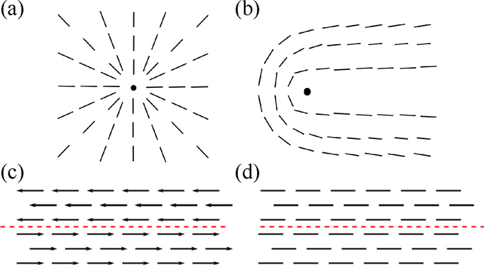 Fig. 1 Representation of topological defects and vector fields(a)one typical example of a 1-defect; (b)one typical example of a 1/2-defect; (c)a vector field with anti-parallel director on each side of the red-dashed line; (d)the line field corresponding to the vector field on the left
 下载:
全尺寸图片
The aim of this paper is twofold. First, we demonstrate that, there exists significant discrepancy between the Oseen-Frank model and Landau-de Gennes model in the transition dynamics for nematic liquid crystals confined in a two-dimension(2D)square well. While the liquid crystal configuration of the starting and ending point of the transition are both orientable line field, a non-orientable configuration that contains half-integer defects appear during the transition process, as predicted by the Landau-de Gennes model. The Oseen-Frank model predicts another pathway because it does not allow half-integer defects. Then, trying to fix this problem and restore the head-to-tail symmetry in the vector model, we replace the standard Laplacian operator in the time-dependent Euler Lagrange equation with the so-called inner-product weighted Laplacian. The new dynamical model with this anisotropic diffusion can predict half-integer defects and a transition pathway like that of the Landau-de Gennes model.
The rest of the paper is organized as follows. In section 2, we review some classical vector and tensor models for nematic liquid crystals. In section 3, we compare the equilibrium and dynamical behavior of the bistable planar liquid crystal well predicted by different models. In section 4, we propose the inner-product weighted Laplacian and show that it leads to anisotropic diffusion dynamics that respect the head-to-tail symmetry. The connections of the anisotropic diffusion operator to the graph Laplacian and the discrete Lebwohl-Lasher model are discussed in section 5 and conclusion is made in section 6.
1. Vector and tensor models of liquid crystals
The simplest continuum theory for nematic liquid crystals is the Oseen-Frank theory [7]. In the domain Ω where the liquid crystals occupy, the order parameter of the Oseen-Frank model is a unit vector director field n = n (x), representing the average alignment of local liquid crystal molecules. The Oseen-Frank free energy density is a quadratic function of the gradient of n, which gives the free energy functional
$$ \begin{gathered} I_{\mathrm{OF}}[\boldsymbol{n}]= \\ \frac{1}{2} \int_{\varOmega}\left(k_1(\nabla \cdot \boldsymbol{n})^2+k_2(\boldsymbol{n} \cdot \nabla \times \boldsymbol{n})^2+k_3(\boldsymbol{n} \times \nabla \times \boldsymbol{n})^2\right) \mathrm{d} \boldsymbol{x}, \end{gathered} $$ (1) here the elastic constants $ k_1, k_2 \text { and } k_3$ are associated with the director's splay, twist, and bend distortions. In the one-constant approximation for which $ k_1=k_2= k_3=k$, the Oseen-Frank energy reduced to
$$ I_{\mathrm{OF}}[\boldsymbol{n}]=\frac{k}{2} \int_{\varOmega}|\nabla \boldsymbol{n}|^2 \mathrm{~d} \boldsymbol{x} . $$ (2) Another more comprehensive vector model for nematic liquid crystals is the Ericksen theory [12]. The Ericksen theory can account for spatially varying of the strength of orientational ordering by bringing in an extra scalar order parameter s. In the simplest setting, the Ericksen free energy as a functional of (s(x), n(x)) is given by
$$ I_{\mathrm{E}}[s, \boldsymbol{n}]=\int_{\varOmega} W(s, \nabla s, \boldsymbol{n}, \nabla \boldsymbol{n}) \mathrm{d} \boldsymbol{x} . $$ (3) See reference [12] for the specific form of $ W(s, \nabla s, \boldsymbol{n}, \nabla \boldsymbol{n})$ The Ericksen theory is particularly useful in describing defects in liquid crystal as it allows the scalar parameters to go to 0 close to the defects so that the free energy does not blow up.
Following the same logic, we found it appealing to use the so-called penalized Oseen-Frank model [17] for the numerical simulation of nematic liquid crystals with defects. Instead of the unit vector field n(x), now the order parameter is a vector filed p(x), with the free energy given by
$$ I_{p \circ \mathrm{~F}}[\boldsymbol{p}]=\int_{\varOmega} \frac{k}{2}|\nabla \boldsymbol{p}|^2+\frac{\omega}{4}\left(\|\boldsymbol{p}\|^2-1\right)^2 \mathrm{~d} \boldsymbol{x}, $$ (4) here the penalty coefficient ω makes sure that p(x) not far away from unit vector everywhere except for a small subset neat defects. Mathematically, the penalized Oseen-Frank model can be considered as a special case of the Ericksen model. In this paper we will use this model for its simplicity and robustness in handling defects.
A third approach is the Landau-de Gennes theory that use a matrix order parameter Q [7].Q is a traceless and symmetric matrix which will be referred as the Q-tensor. The simplest commonly used form of the Landau-de Gennes energy functional is
$$ I_{\mathrm{LdG}}[\boldsymbol{Q}]=\int_{\varOmega} \frac{L}{2}|\nabla \boldsymbol{Q}|^2-\frac{a}{2} \operatorname{tr}\left(\boldsymbol{Q}^2\right)-\frac{b}{3} \operatorname{tr}\left(\boldsymbol{Q}^3\right)+\frac{c}{4} \operatorname{tr}\left(\boldsymbol{Q}^2\right)^2 \mathrm{~d} \boldsymbol{x}, $$ (5) where $ a, b>0 \text { and } c>0$ are temperature and material dependent constants and L > 0 is the elastic constant.
In this paper, we will restrict out attention to 2D models, meaning $ \varOmega \subset \mathbf{R}^2 \text { and } \boldsymbol{n}=\left(n_1, n_2\right)$ is a 2D vector field. The 2D Q-tensor
$$ \boldsymbol{Q}=\left(\begin{array}{cc} q_1 & q_2 \\ q_2 & -q_1 \end{array}\right) $$ (6) is a 2 × 2 matrix with two degrees-of-freedom.Q can also be expressed by a scalar parameter s and unit vector n as
$$ \boldsymbol{Q}=2 s(\boldsymbol{n} \boldsymbol{n}-\boldsymbol{I}), $$ (7) where I is the 2 × 2 identity matrix. Expressing n in terms of an angle θ in the xy-plane by n = (cosθ, sinθ) one can readily check that
$$ q_1=s \cos (2 \theta), \quad q_2=s \sin (2 \theta) . $$ (8) We also have
$$ \operatorname{tr} \boldsymbol{Q}=\operatorname{tr} \boldsymbol{Q}^3=0, \quad \operatorname{tr} \boldsymbol{Q}^2=2 s^2 . $$ (9) Substitute equations(6), (8)and(9)into equation(5)gives(after dropping a constant)
$$ I_{\mathrm{IdG}}[\boldsymbol{Q}]=\int_{\varOmega} L\left(\left|\nabla q_1\right|^2+\left|\nabla q_2\right|^2\right)+c\left(q_1^2+q_2^2-s_0^2\right)^2 \mathrm{~d} \boldsymbol{x}, $$ (10) where $ s_0=\sqrt{a / 2 c}$.
In the special case that s is constant everywhere, the 2D Landau-de Gennes free energy equation(10)can be written as(up to a constant)
$$ I_{\mathrm{LdG}}[\theta]=4 s^2 L \int_{\varOmega}|\nabla \theta|^2 \mathrm{~d} \boldsymbol{x} . $$ (11) Note that equation(2)can also be written as
$$ I_{\mathrm{OF}}[\theta]=\frac{k}{2} \int_{\varOmega}|\nabla \theta|^2 \mathrm{~d} \boldsymbol{x} . $$ (12) Thus, the Landau-de Gennes model in the special case of constant scalar order parameter is equivalent to the Oseen-Frank model. However, it is important to note that this equivalence holds only if for the tensor fieldQ(x), one can assign a field θ(x) that is smooth enough so that equation(11)does not diverge. Unfortunately, it is not always possible to do so due to the issue of non-orientability, which is discussed in detail in [13, 18]. To see this, we note from equation(7)that for s > 0 constant Q is a line field. For any x, there can be an association with either n(x) or − n(x). In fact, there exists continuous line fields that cannot be assigned with a vector field without creating discontinuity. Moving from Oseen-Frank model to Ericksen model by allowing s → 0 near defects does not fully solve the non-orientability issue. One example is the 1/2-defect(see [13, 18]). One typical example of a 1/2-defect is shown in figure 1(a), whereas a 1-defect is shown in figure 1(b). The notation of an m-defect refers to the winding number of the orientational field around the defect. For tensor models like the Landau-de Gennes model, m can be either an integer or a half-integer plus an integer(e.g., m=1/2). The consensus from the literature is that the Oseen-Frank model and Ericksen model cannot predict defects with half-integer strength. One obvious reason is that, for the case shown in figure 1(c), the elastic energy is non-zero in the Oseen-Frank model and Ericksen model while it is zero in the Landau-de Gennes model as it should be because of the head-to-tail symmetry(figure 1(c)). Basically, if one must deal with the $ \nabla \boldsymbol{n}$ term in the free energy functional of a vector model, then it will encounter problems when describing configurations such as the one shown in figure 1(d), which often occurs when assigning a vector field to a line field containing half-integer defects.
2. Bistable planar liquid crystal well
In this section we demonstrate that, significant discrepancy between the vector model and tensor model may exist if the head-to-tail symmetry is not respected in the vector model. We consider nematic liquid crystals confined in a shallow square well subject to planar boundary constraint. The depth of the well is so small that it is sufficient to consider a 2D director field n(or 2D tensor field Q)on
$$ \varOmega=\left\{(x, y) \in \mathbf{R}^2|0 \leqslant|x| \leqslant l, 0 \leqslant|y| \leqslant l\} .\right. $$ (13) To mimic the planar boundary constraint, we consider the weak-anchoring condition in which a penalty term is added to the total free energy forcing the liquid molecules to lie in the tangent direction at the boundary. In the Landau-de Gennes model, the boundary energy is
$$ W_{\mathrm{LG}}=\int_{\varOmega} \eta \boldsymbol{v} \cdot \boldsymbol{Q} \boldsymbol{v} \mathrm{d} l, $$ (14) where v is the outward unit-normal vector on ∂Ω, and η is a constant that represents the anchoring strength on ∂Ω. Under this boundary constraint, the confined nematic liquid crystals exhibit multiple equilibrium states. Figure 2(a) depicts one of the so-called diagonal solutions of the system in which the liquid crystals tend to align along the main diagonal direction of the square. Rotating this solution by 90-degree we obtain another diagonal solution in which alignment direction is along the secondary diagonal. Both diagonal solutions are stable. There is another type of equilibrium state in which the vector roughly rotates like an alphabet "U" shape(not shown here, see [19]). Starting from random initial condition and following the gradient flow of the system, we could observe various kinds of defects-containing transit state before the system finally reaching equilibrium. One of the transit states is shown in figure 2(b), in which there exist one 1/2-defect and one -1/2-defect inside the square. In figure 2(b), dark gray color corresponds to places where the value of $ s=\sqrt{q_1^2+q_2^2}$ is small. The parameters are $ \omega=1 \times 10^6, \eta=2500, \varepsilon=0$.
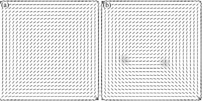 Fig. 2 Prediction and dynamics of nematic liquid crystals via the Landau-de gennes model(a)diagonal configuration predicted by the Landau-de Gennes model for the bistable planar liquid crystal well; (b)a transit state obtained using the timedependent Euler-Lagrange equation equation(18)下载:
全尺寸图片
Under external forcing, the system may undergo a transition from one diagonal configuration to another. To study this type of switching process, we consider the following external potential
$$ E_{\mathrm{LdG}}=\int_{\Omega} \varepsilon \boldsymbol{e} \cdot \boldsymbol{Q} \boldsymbol{e} \mathrm{d} \boldsymbol{x} . $$ (15) Here the coefficient ε controls the strength of the external potential. We choose e = (1, 1) so that the external potential tends to align the liquid crystal molecules along the secondary diagonal direction. Now the total free energy of the system is
$$ \begin{gathered} F_{\mathrm{LdG}}^{\text {total }}=I_{\mathrm{LdG}}+W_{\mathrm{LdG}}+E_{\mathrm{LdG}}= \\ \int_{\varOmega}\left\{L\left(\left|\nabla q_1\right|^2+\left|\nabla q_2\right|^2\right)+c\left(q_1^2+q_2^2-s_0^2\right)^2+\right. \\ \left.\varepsilon\left(q_1 \cos \left(2 \theta_e\right)+q_2 \sin \left(2 \theta_e\right)\right)\right\} \mathrm{d} x+ \\ \int_{\partial \varOmega} \eta\left(q_1 \cos \left(2 \theta_v\right)+q_2 \sin \left(2 \theta_v\right)\right) \mathrm{d} l, \end{gathered} $$ (16) where $\boldsymbol{v}=\left(\cos \theta_v, \sin \theta_v\right) $ and $ \boldsymbol{e}=\left(\cos \theta_e, \sin \theta_e\right)$.
We non-dimensionalize the system by defining $ \tilde{x}=x / l \text { and } \tilde{y}=y / l$ so that the simulation domain $ \varOmega$ becomes $ \tilde{\varOmega}=[0, 1] \times[0, 1]$. Let $ \tilde{q}_1=q_1 / s_0, \tilde{q}_2=q_2 / s_0$, $ \tilde{\omega}=c l^2 / L, \quad \tilde{\eta}=\eta l / s_0 L, \quad \tilde{\varepsilon}=\varepsilon l^2 / s_0 L$, and $ \tilde{F}_{\mathrm{LdG}}^{\text {total }}= F_{\mathrm{IdG}}^{\text {total }} / s_0^2 L$. In terms of new variables, after dropping the tilde symbols for simplicity, the dimensionless total free energy is
$$ \begin{aligned} F_{\mathrm{IdG}}^{\text {total }}= & \int_{\varOmega}\left\{\left(\left|\nabla q_1\right|^2+\left|\nabla q_2\right|^2\right)+\omega\left(q_1^2+q_2^2-1\right)^2+\right. \\ & \left.\varepsilon\left(q_1 \cos \left(2 \theta_e\right)+q_2 \sin \left(2 \theta_e\right)\right)\right\} \mathrm{d} x+ \\ & \int_{\partial \varOmega} \eta\left(q_1 \cos \left(2 \theta_v\right)+q_2 \sin \left(2 \theta_v\right)\right) \mathrm{d} l . \end{aligned} $$ (17) The dynamics of the system is described by the gradient flow, i.e., the following time-dependent Euler-Lagrange equation
$$ \left\{\begin{array}{l} \partial_t q_1=\Delta q_1-\omega\left(q_1^2+q_2^2-1\right) q_1-\varepsilon \cos \left(2 \theta_e\right), \text { in } \varOmega, \\ \partial_t q_2=\Delta q_2-\omega\left(q_1^2+q_2^2-1\right) q_2-\varepsilon \sin \left(2 \theta_e\right), \text { in } \varOmega, \\ \partial_t q_1=-\frac{\partial q_1}{\partial v}-\eta \cos \left(2 \theta_v\right), \text { on } \partial \varOmega, \\ \partial_t q_2=-\frac{\partial q_2}{\partial v}-\eta \sin \left(2 \theta_v\right), \text { on } \partial \varOmega . \end{array}\right. $$ (18) We numerically solve equation(18)using finite difference scheme over a uniform mesh with 100 × 100. The Laplacian is discretized using five-point central difference scheme. The directional derivative on the boundary is treated using the method of lines. Explicit Euler scheme is used for time integration. The initial condition is given by figure 2(a).
For the parameters specified in the figure caption, the transition driven by the external potential follows a pathway as shown in figure 3. Dark gray color corresponds to places where the value of $ s= \sqrt{q_1^2+q_2^2}$ is small. The parameters are $ \omega=1 \times 10^6, \eta=2500, \varepsilon=500$. At first, molecules close to the edge reorientate, causing the line field near the two diagonals to distort. The two distorted strips gradually separate in the middle of the square. Next, we can observe that the two distorted strips break in the middle, forming four half-integer defects(two of them are index 1/2 and the other two index − 1/2). In our numerical experiment we found that, to make the two distorted strips to separate and break, the strength of the external potential is the key parameter while other parameters are less relevant. A too weak external potential cannot separate the distorted strips, or if it can, the separated strips may not break but slide to the edges instead. On the other hand, if the external potential is too strong, the transition will follow a different pathway in which the distorted strips detach from the square vertex and retract to the center of the square and vanish. To make sure that the predicted dynamical behavior is not a numerical artifact, we carried out simulation with increases spatial and temporal resolution and found that the same dynamical behavior persists.
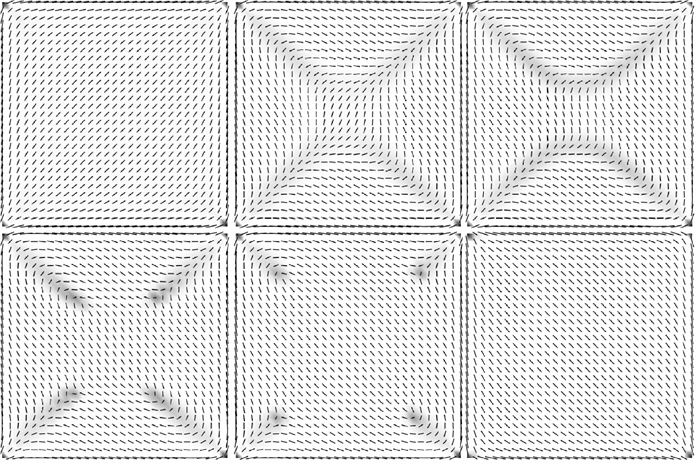 Fig. 3 Transition path for the Landau-de gennes model for the bistable planar liquid crystal well下载:
全尺寸图片
We have seen that, during the transition dynamics, even though both the starting and ending point of the transition pathway are orientable, ±1/2-defects can appear inside the square, which makes the line field transiently non-orientable. Because it is believed that the Oseen-Frank model cannot predict configurations containing ±1/2-defects inside the square, we speculate that the transition process predicted by the Oseen-Frank model will follow a different path that does not contain any half-integer defect inside the square. To make a comparison between the Oseen-Frank model and Landau-de Gennes model, we consider the following planar boundary constraint and external potential in the penalized-Oseen-Frank model. The boundary constraint is enforced by the penalty term
$$ W_{p \mathrm{OF}}=\int_{\partial \varOmega} \frac{\eta}{2}(\boldsymbol{n} \cdot \boldsymbol{v})^2 \mathrm{~d} l, $$ (19) and the external potential is given by
$$ E_{p \mathrm{OF}}=\int_{\partial \varOmega} \frac{\varepsilon}{2}(\boldsymbol{n} \cdot \boldsymbol{e})^2 \mathrm{~d} \boldsymbol{x} . $$ (20) The total free energy is
$$ \begin{gathered} F_{p \mathrm{OF}}^{\text {Loal }}=I_{p \mathrm{OF}}+W_{p \mathrm{OF}}+E_{p \mathrm{OF}}= \\ \int_{\varOmega}\left\{\frac{k}{2}|\nabla \boldsymbol{p}|^2+\frac{\omega}{4}\left(\|\boldsymbol{p}\|^2-1\right)^2+\frac{\varepsilon}{2}(\boldsymbol{n} \cdot \boldsymbol{e})^2\right\} \mathrm{d} \boldsymbol{x}+ \\ \int_{\partial \varOmega} \frac{\eta}{2}(\boldsymbol{n} \cdot \boldsymbol{v})^2 \mathrm{~d} l . \end{gathered} $$ (21) Again, we non-dimensionalize the system by defining $ \tilde{x}=x / l \text { and } \tilde{y}=y / l \text { and } \varOmega$ becomes $ \tilde{\varOmega}= [0, 1] \times[0, 1] \cdot \tilde{\omega}=\omega l^2 / L, \tilde{\eta}=\eta l / k, \tilde{\varepsilon}=\varepsilon l^2 / k, \text { and } \tilde{F}_{p \text{OF}}^{\text {total }}= F_{p \mathrm{OF}}^{\text {total }} / k$. In terms of new variables, after dropping the tilde symbols for simplicity, the dimensionless total free energy becomes
$$ \begin{gathered} F_{p \mathrm{OF}}^{\text {total }}=\int_{\varOmega}\left\{\frac{1}{2}|\nabla \boldsymbol{p}|^2+\frac{\omega}{4}\left(\|\boldsymbol{p}\|^2-1\right)^2+\frac{\varepsilon}{2}(\boldsymbol{n} \cdot \boldsymbol{e})^2\right\} \mathrm{d} \boldsymbol{x}+ \\ \int_{\partial \varOmega} \frac{\eta}{2}(\boldsymbol{n} \cdot \boldsymbol{v})^2 \mathrm{~d} l . \end{gathered} $$ The corresponding time-dependent Euler-Lagrange equation is
$$ \left\{\begin{array}{l} \partial_t p_1=\Delta p_1-\omega\left(p_1^2+p_2^2-1\right) q_1-\varepsilon(\boldsymbol{p} \cdot \boldsymbol{e}) p_1, \text { in } \varOmega , \\ \partial_t p_2=\Delta p_2-\omega\left(p_1^2+p_2^2-1\right) q_2-\varepsilon(\boldsymbol{p} \cdot \boldsymbol{e}) p_2, \text { in } \varOmega, \\ \partial_t p_1=-\frac{\partial p_1}{\partial \boldsymbol{v}}+\frac{\partial p_1}{\partial \boldsymbol{u}}-\eta(\boldsymbol{p} \cdot \boldsymbol{e}) p_1, \text { on } \partial \varOmega, \\ \partial_t p_2=-\frac{\partial p_2}{\partial \boldsymbol{v}}+\frac{\partial p_2}{\partial \boldsymbol{u}}-\eta(\boldsymbol{p} \cdot \boldsymbol{e}) p_2, \text { on } \partial \varOmega, \end{array}\right. $$ (23) where $ \boldsymbol{v}=\left(v_1, v_2\right)$ is the outward unit-normal vector on $ \partial \varOmega, \text { and } \boldsymbol{u}=\left(-v_2, v_1\right)$ is the tangent vector of $\boldsymbol{v}$.
First we set the external potential to 0 and simulate the gradient flow equation(23). Similar to the Landau-de Gennes model, for sufficient long time the system can reach equilibrium state as shown in figure 4(a). During the simulation, we may observe configurations with ±1-defects, as shown in figure 4(b). This is different from figure 2(b).
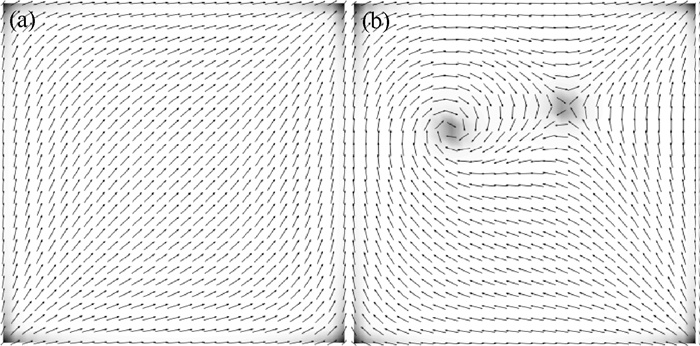 Fig. 4 Dynamics of nematic liquid crystals via the Oseen-Frank model(a)diagonal configuration predicted by the Oseen-Frank model for the bistable planar liquid crystal well; (b)a transit state obtained using the time-dependent Euler-Lagrange equation equation(23)下载:
全尺寸图片
Next, we study the transition from one diagonal solution to another diagonal solution driven by external potential. Starting from the initial condition given by figure 5(a), we simulate equation(23)with parameters specified in the figure legend. The transition pathway is shown in figure 5. Unlike the prediction made by the Landau-de Gennes model, the Oseen-Frank model predicts a transition path that does not involving any creation of half-integer defect inside the square. Instead, the distorted lines do not break up in the middle but retract and vanish at the boundary.
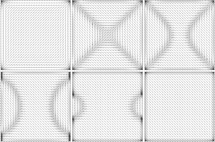 Fig. 5 Transition path for the Oseen-Frank model for the bistable planar liquid crystal well下载:
全尺寸图片
3. Anisotropic diffusion dynamics for the modified Oseen-Frank model
The above numerical results demonstrate a significant discrepancy between the Oseen-Frank model and the Landau-de Gennes model, especially when used to predict the dynamics of a nematic liquid crystals. The incapability of the Oseen-Frank model to predict half-integer defects is a result of the fact that the head-to-tail symmetry is not fulfilled in the model.
As shown in the above example, the discrepancy between the vector model and tensor model in predicting defect patterns is caused by the lack of head-to-tail symmetry in the vector model. For situations such as the one illustrated in figure 1(c), it is difficult to explicitly handle terms like $ \nabla \boldsymbol{n}$ because n is not everywhere differentiable(see figure 8 and discussion in section 4.2). In the following we present a remedy that can restore the head-to-tail symmetry in the vector model.
Formally, we define the 2D inner-product weighted Laplacian for a vector field $ \boldsymbol{p}(x, y), (x, y) \in \varOmega \subset \mathbf{R}^2$ as
$$ \Delta^{i w} \boldsymbol{p}=\lim\limits_{h \rightarrow 0} \frac{1}{h^2}\left[\begin{array}{c} \left(\boldsymbol{p} \cdot \boldsymbol{p}_1\right) \boldsymbol{p}_1+\left(\boldsymbol{p} \cdot \boldsymbol{p}_2\right) \boldsymbol{p}_2+\left(\boldsymbol{p} \cdot \boldsymbol{p}_3\right) \boldsymbol{p}_3+ \\ \left(\boldsymbol{p} \cdot \boldsymbol{p}_4\right) \boldsymbol{p}_4-\sum\limits_{i=1}^4\left(\boldsymbol{p} \cdot \boldsymbol{p}_i\right) \boldsymbol{p} \end{array}\right], $$ (24) where
$$ \begin{gathered} \boldsymbol{p}=(x, y), \boldsymbol{p}_1=(x+h, y), \boldsymbol{p}_2=(x-h, y), \\ \boldsymbol{p}_3=(x, y+h), \boldsymbol{p}_4=(x, y-h), \end{gathered} $$ $ \Delta^{i w}$ is a non-linear operator on vector field p. If p is continuous differentiable unit vector field, p·pi approaches 1 as h → 0, thus the standard Laplacian
$$ \Delta \boldsymbol{n}=\lim\limits_{h \rightarrow 0} \frac{1}{h^2}\left[\boldsymbol{n}_1+\boldsymbol{n}_2+\boldsymbol{n}_3+\boldsymbol{n}_4-4 \boldsymbol{n}\right], $$ (25) for unit vector n is recovered.
The idea behind the inner-product weighted Laplacian comes from the Lebwohl-Lasher model for unit vectors located on a 2D lattice, for which the free energy takes the following form
$$ F_{L L}[\boldsymbol{n}]=-\frac{1}{2} J \sum\limits_{\{l, m\}_{n n}}\left[\left(\boldsymbol{n}_l, \boldsymbol{n}_m\right)^2-1\right], $$ (26) where the summation is taken over nearest neighbors(nn)on the lattice.J is the interaction strength. For J = 1, the free energy density can be written as
$$ \begin{aligned} & f_{L L}\left(\boldsymbol{n}_{i j}\right)=-\frac{1}{2}\left[\left(\boldsymbol{n}_{i j}, \boldsymbol{n}_{i+1, j}\right)^2+\left(\boldsymbol{n}_{i j}, \boldsymbol{n}_{i-1, j}\right)^2+\right. \\ & \left.\left(\boldsymbol{n}_{i j}, \boldsymbol{n}_{i, j-1}\right)^2+\left(\boldsymbol{n}_{i j}, \boldsymbol{n}_{i, j+1}\right)^2-4\left(\boldsymbol{n}_{i j}, \boldsymbol{n}_{i j}\right)^2\right]. \end{aligned} $$ (27) Taking the derivative of $ f_{L L}\left(\boldsymbol{n}_{i j}\right)$ with respect to the element of $ \boldsymbol{n}_{i j}=\left(n_{i j}^{(1)}, n_{i j}^{(2)}\right)$, we get
$$ \begin{aligned} & \frac{\partial f\left(\boldsymbol{n}_{i j}\right)}{\partial n_{i j}^{(1)}}=-\left[\left(\boldsymbol{n}_{i j} \cdot \boldsymbol{n}_{i+1, j}\right) n_{i+1, j}^{(1)}+\left(\boldsymbol{n}_{i j} \cdot \boldsymbol{n}_{i-1, j}\right) n_{i-1, j}^{(1)}+\right. \\ & \left.\left(\boldsymbol{n}_{i j} \cdot \boldsymbol{n}_{i, j-1}\right) n_{i, j-1}^{(1)}+\left(\boldsymbol{n}_{i j} \cdot \boldsymbol{n}_{i, j+1}\right) n_{i, j+1}^{(1)}-4 n_{i j}^{(1)}\right] \\ & \frac{\partial f\left(\boldsymbol{n}_{i j}\right)}{\partial n_{i j}^{(2)}}=-\left[\left(\boldsymbol{n}_{i j} \cdot \boldsymbol{n}_{i+1, j}\right) n_{i+1, j}^{(2)}+\left(\boldsymbol{n}_{i j} \cdot \boldsymbol{n}_{i-1, j}\right) n_{i-1, j}^{(2)}+\right. \\ & \left.\left(\boldsymbol{n}_{i j} \cdot \boldsymbol{n}_{i, j-1}\right) n_{i, j-1}^{(2)}+\left(\boldsymbol{n}_{i j} \cdot \boldsymbol{n}_{i, j+1}\right) n_{i, j+1}^{(2)}-4 n_{i j}^{(2)}\right] . \end{aligned} $$ (28) We can think of the terms on the right-hand-side of equation(28)as a discretized Laplacian, with the four inner products $ \boldsymbol{n}_{i j} \cdot \boldsymbol{n}_{i+1, j}, \boldsymbol{n}_{i j} \cdot \boldsymbol{n}_{i-1, j}, \boldsymbol{n}_{i j} \cdot \boldsymbol{n}_{i, j-1}$ and $ \boldsymbol{n}_{i j} \cdot \boldsymbol{n}_{i, j+1}$ to be the weight coefficients similar to those in equation(24).
As we have shown previously that the Lebwohl-Lasher model can predict half-integer defects in the planar bistable well example, we expect that using the inner-product weighted Laplacian can restore head-to-tail symmetry in the vector model. To this end, we replace the standard Laplacian in the original time-dependent Euler-Lagrange equation in equation(23)with the inner-product weighted Laplacian. In the planar bistable well model, with the same tangent anchoring condition equation(19)and external potential equation(20), the dynamics of vector field p is given by
$$ \left\{\begin{array}{l} \partial_t p_1=\Delta^{\mathrm{iw}} p_1-\omega\left(p_1^2+p_2^2-1\right) q_1-\varepsilon(\boldsymbol{p} \cdot \boldsymbol{e}) p_1, \text { in } \varOmega, \\ \partial_t p_2=\Delta^{\mathrm{iw}} p_2-\omega\left(p_1^2+p_2^2-1\right) q_2-\varepsilon(\boldsymbol{p} \cdot \boldsymbol{e}) p_2, \text { in } \varOmega, \\ \partial_t p_1=-\frac{\partial p_1}{\partial \boldsymbol{v}}+\frac{\partial p_1}{\partial \boldsymbol{u}}-\eta(\boldsymbol{p} \cdot \boldsymbol{e}) p_1, \text { on } \partial \varOmega, \\ \partial_t p_2=-\frac{\partial p_2}{\partial \boldsymbol{v}}+\frac{\partial p_2}{\partial \boldsymbol{u}}-\eta(\boldsymbol{p} \cdot \boldsymbol{e}) p_2, \text { on } \partial \varOmega . \end{array}\right. $$ (29) Using the new dynamical model in our numerical simulation, we obtain the diagonal solution as one equilibrium state(figure 6(a)). Unlike the penalized Oseen-Frank model(figure 4(a)), now many nearby vectors are anti-parallel with each other. Moreover, in transit states before the system reaches equilibrium, we can observe half-integer defects(figure 6(b)). We also use the new model to simulate the transition process(figure 7). It shows that the transition dynamics is very similar to the one predicted by the Landau-de Gennes model, in which four ±1/2-defects forms inside the square. Thus, by replacing the standard Laplacian by the inner-product weighted Laplacian, the head-to-tail symmetry can be restored in the dynamical model.
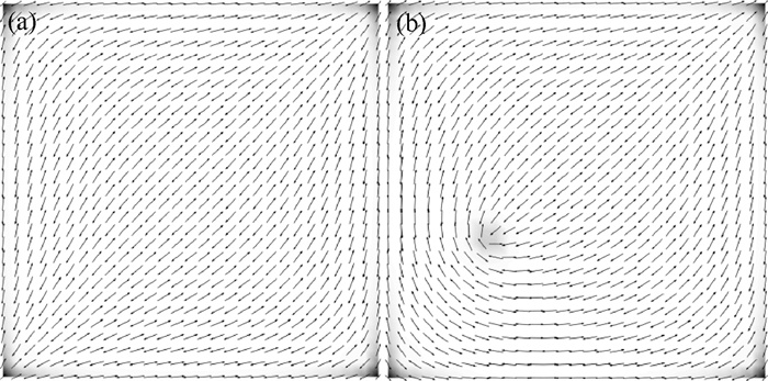 Fig. 6 Dynamics of nematic liquid crystals via the Oseen-Frank model(a)diagonal configuration predicted by the modified Oseen-Frank model for the bistable planar liquid crystal well; (b)a transit state obtained using the time-dependent Euler-Lagrange equation equation(29)下载:
全尺寸图片
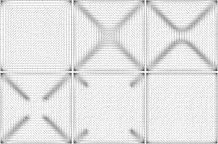 Fig. 7 Transition path for the modified Oseen-Frank model with inner-product weighted Laplacian for the bistable planar liquid crystal well下载:
全尺寸图片
4. Discussions
4.1 The free energy of the new model
The inner-product weighted Laplacian as given in equation(24)can serve as a convenient way to numerically restore head-to-tail symmetry in the modified Oseen-Frank vector model. One intriguing question that follows is, what is the corresponding free energy functional for such an anisotropic diffusion dynamic. In the previous section we show that the inner-product weighted Laplacian has a close relationship with the Lebwohl-Lasher model. In the following we show that, if n(x) is smooth, then formally the continuous limit of the Lebwohl-Lasher when the grid size h → 0 is Oseen-Frank model. To see this, note that the energy per single site in the Lebwohl-Lasher model is
$$ \begin{gathered} f_{L L}\left(\boldsymbol{n}_{i j}\right)=-\frac{1}{2}\left[\left(\boldsymbol{n}_{i j}, \boldsymbol{n}_{i+1, j}\right)^2+\left(\boldsymbol{n}_{i j}, \boldsymbol{n}_{i-1, j}\right)^2\right. \\ \left.+\left(\boldsymbol{n}_{i j}, \boldsymbol{n}_{i, j-1}\right)^2+\left(\boldsymbol{n}_{i j}, \boldsymbol{n}_{i, j+1}\right)^2-4\right] . \end{gathered} $$ (30) Because n is smooth, we apply Taylor expansion for n and neglect the $ O\left(h^2\right)$ term, which gives
$$ \begin{aligned} \left(\boldsymbol{n}_{i j}, \boldsymbol{n}_{i+1, j}\right)^2= & {\left[\boldsymbol{n}_{i j} \cdot\left(\boldsymbol{n}_{i j}+h \frac{\boldsymbol{n}_{i+1, j}-\boldsymbol{n}_{i j}}{h}\right)\right]^2=} \\ & {\left[1+h \boldsymbol{n}_{i j} \cdot \frac{\boldsymbol{n}_{i+1, j}-\boldsymbol{n}_{i j}}{h}\right]^2 \approx } \\ & 1+2 h \boldsymbol{n}_{i j} \cdot \frac{\boldsymbol{n}_{i+1, j}-\boldsymbol{n}_{i j}}{h}, \end{aligned} $$ (31) and
$$ \begin{gathered} f_{L L}\left(\boldsymbol{n}_{i j}\right)= \\ -\frac{1}{2}\left[2 h^2 \boldsymbol{n}_{i j} \cdot \frac{\boldsymbol{n}_{i+1, j}+\boldsymbol{n}_{i-1, j}+\boldsymbol{n}_{i, j-1}+\boldsymbol{n}_{i, j+1}-4 \boldsymbol{n}_{i j}}{h^2}\right]= \\ -h^2 \boldsymbol{n}_{i j} \cdot \Delta \boldsymbol{n}_{i j} . \end{gathered} $$ (32) In the limit of h → 0, the energy density becomes
$$ f_{L L}(\boldsymbol{n}(\boldsymbol{x}))=\lim\limits_{h \rightarrow 0} \frac{f_{L L}\left(\boldsymbol{n}_{i j}\right)}{h^2}=-\boldsymbol{n}(\boldsymbol{x}) \cdot \Delta \boldsymbol{n}(\boldsymbol{x})=|\nabla \boldsymbol{n}(\boldsymbol{x})|^2, $$ which equals to the energy density in the Oseen-Frank model(equation(2)). Thus, if the vector field p can be partitioned into a finite set of simply connected regions so that p is continuous inside each region, then we expect that the free energy functional for each region has the same form as given by equation(4), and so does their sum. Although a rigorous mathematical formulation is missing, our guess is that the free energy functional corresponding to the anisotropic diffusion still takes the same form as equation(4), but with p lives in an enlarged functional space, say, $ W_1^p(\varOmega)$.
4.2 Another attempt that does not work
We made another attempt to restore the head-to-tail symmetry in the Oseen-Frank model by re-defining the discretized gradient operator in a way described as follows. For two vectors on adjacent grids, say, $ \boldsymbol{p}(x, y) \text { and } \boldsymbol{p}(x+h, y)$, where h is the grid length, we compute two divergences: one using the original vectors and the other with one vector rotated by π. That is
$$ \begin{aligned} & \frac{\Delta_{+} \boldsymbol{p}(x, y)}{\Delta x}=\boldsymbol{p}(x+\Delta x, y)-\boldsymbol{p}(x, y), \\ & \frac{\Delta_{-} \boldsymbol{p}(x, y)}{\Delta x}=-\boldsymbol{p}(x+\Delta x, y)-\boldsymbol{p}(x, y) . \end{aligned} $$ (33) Among the two we choose the one with smaller absolute value as the effective gradient, i.e.
$$ \frac{\Delta \boldsymbol{p}(x, y)}{\Delta x}= \begin{cases}\frac{\Delta_{+} \boldsymbol{p}(x, y)}{\Delta x}, & \text { if }\left|\frac{\Delta_{+} \boldsymbol{p}(x, y)}{\Delta x}\right| \leqslant\left|\frac{\Delta_{-} \boldsymbol{p}(x, y)}{\Delta x}\right|, \\ \frac{\Delta_{-} \boldsymbol{p}(x, y)}{\Delta x}, & \text { otherwise. }\end{cases} $$ (34) By doing so, two anti-parallel adjacent vectors will contribute zero elastic energy to the system because their effective gradient is zero. With this property, one can check that configurations containing half-integer defects will have the same energy under the Landau-de Gennes model and the Oseen-Frank model with the modified gradient operator. However, in our numerical simulation we found that, the energy landscape associated with the new gradient operator is so rough that it is highly likely for the system to get trapped at some peculiar configurations like the one shown in figure 8.
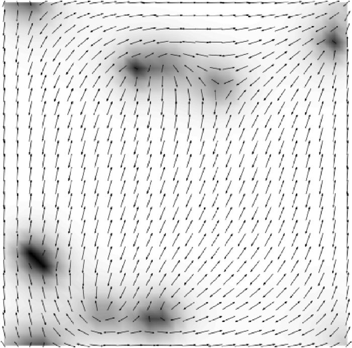 Fig. 8 Transit state for the model with modified gradient in the Oseen-Frank model下载:
全尺寸图片
Figure 9 explains why the modified gradient approach fails. Consider two adjacent directors as shown in figure 9(a). When computing the modified gradient for director p1 with respect to director p2, the gray dashed director will be chosen as it is the one with smaller gradient value. As a result, p1 tends to rotate clockwise to the direction parallel to p2, which is what we needed. When an extra adjacent director p3 is added, one can check that when θ is close to π/2, the modified gradient will use the dashed vector(-p1)for both p2 and p3. As a result, now p1 tends rotate counter-clockwise towards the y-axis, which is not what we want. Under head-to-tail symmetry, what we expect is that the line segment will rotate counter-clockwise towards the y-axis when ϕ > π/4, and rotate clockwise towards the x-axis when ϕ < π/4.
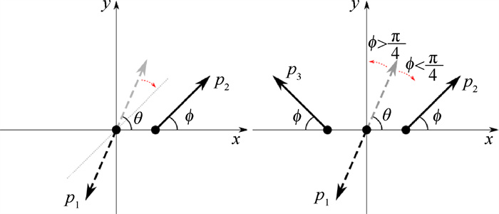 Fig. 9 An illustration of why equation(34)does not work下载:
全尺寸图片
What will the inner-product weighted Laplacian do in these circumstances?For the case in figure 9(a) it coincides with the previous case, that is, orientating the line segment of p1 clockwise. For the case in figure 9(b), the free energy of p1(keeping the other two directors fixed)under the inner-product weighted Laplacian is
$$ \begin{array}{c} f(\theta)=\boldsymbol{p}_1 \cdot \Delta^{i w} \boldsymbol{p}_1= \\ \binom{\cos \theta}{\sin \theta} \cdot\binom{\cos \phi(\cos (\theta-\phi)+\cos (\theta+\phi))-2 \cos \theta}{\sin \phi(\sin (\theta-\phi)+\sin (\theta+\phi))-2 \sin \theta}= \\ -2 \cos ^2 \theta \sin ^2 \phi-2 \sin ^2 \theta \cos ^2 \phi= \\ \cos (2 \theta) \cos (2 \phi). \end{array} $$ (35) From equation(35)we can see that, if ϕ > π/4, θ will increase to π/2 to minimize the f(θ), and if ϕ < π/4, θ will decrease to 0. This is exactly what we expected.
4.3 Relation with the graph Laplacian
The inner-product weighted Laplacian equation(24)can be understood as the limit of a special kind of graph Laplacian defined on a network for which the nodes are vector-valued. The proximity between a pair of neighboring nodes is replaced by the inner-product of the vectors on the two nodes: when the two vectors are parallel with each other, the interaction between the two nodes become strong; and when the two vectors are anti-parallel with each other, the interaction becomes "negative"(which is not common in conventional graph Laplacians). In some sense this proximity can be viewed as a metric defined in the space $ \left\{(\boldsymbol{x}, \boldsymbol{p}) \mid \boldsymbol{x} \in \mathbf{R}^2, \boldsymbol{p} \in \mathbf{R}^2\right\}$. It would be interesting to investigate diffusion geometry [20] in it.
The idea of modifying the proximity between a pair of neighboring molecules with their alignment information can also be applied to molecules with different symmetry. For example, figure 10 gives three kinds of molecules whose orientation can be determined by a vector p(as indicated by the arrows in the figure)but with different orders of rotational symmetry m(Trigonal m=3; Square m=4; Pentagonal m=5). One could then define the discretized Laplacian on a regular 2D lattice as
$$ \begin{gathered} \Delta^m \boldsymbol{p}=d\left(\boldsymbol{p}, \boldsymbol{p}_1\right) \boldsymbol{p}_1+d\left(\boldsymbol{p}, \boldsymbol{p}_2\right) \boldsymbol{p}_2+d\left(\boldsymbol{p}, \boldsymbol{p}_3\right) \boldsymbol{p}_3+ \\ d\left(\boldsymbol{p}, \boldsymbol{p}_4\right) \boldsymbol{p}_4-\sum\limits_{i=1}^4 d\left(\boldsymbol{p}, \boldsymbol{p}_i\right) \boldsymbol{p} . \end{gathered} $$ Here the proximity function is defined as
$$ d(\boldsymbol{p}(\boldsymbol{x}), \boldsymbol{p}(\boldsymbol{y}))=|\boldsymbol{p}(\boldsymbol{x})| \cdot|\boldsymbol{p}(\boldsymbol{y})| \cdot \cos \left(\frac{m \theta}{2}\right) . $$ 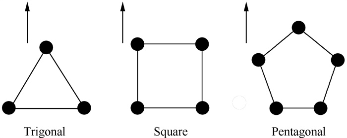 Fig. 10 Molecules with different symmetry下载:
全尺寸图片
Under certain topological constraint, liquid crystals formed by these molecules may also contain different kinds of defects and it would be interesting to compare the above model with other existing models [21].
5. Conclusion
Using the planar bistable well as an example, we demonstrate that there could be significant discrepancy between the Oseen-Frank vector model and the Landau-de Gennes tensor model in their predicted transition dynamics. The reason is that the Oseen-Frank model does not respect the head-to-tail symmetry. As a fix to this deficiency, we propose the inner-product weighted Laplacian Δiw. Using this new Laplacian to replace the standard Laplacian in the time-dependent Euler-Lagrange equation corresponding to the Oseen-Frank model, we found that the head-to-tail symmetry is restored in the modified dynamics. In future it would be interesting to investigate the mathematical properties of the new Laplacian and compare the new vector model with the Landau-de Gennes tensor model in 3D.
-
Fig. 1 Representation of topological defects and vector fields
(a)one typical example of a 1-defect; (b)one typical example of a 1/2-defect; (c)a vector field with anti-parallel director on each side of the red-dashed line; (d)the line field corresponding to the vector field on the left
下载:
全尺寸图片
Fig. 2 Prediction and dynamics of nematic liquid crystals via the Landau-de gennes model
(a)diagonal configuration predicted by the Landau-de Gennes model for the bistable planar liquid crystal well; (b)a transit state obtained using the timedependent Euler-Lagrange equation equation(18)
下载:
全尺寸图片
Fig. 3 Transition path for the Landau-de gennes model for the bistable planar liquid crystal well
下载:
全尺寸图片
Fig. 4 Dynamics of nematic liquid crystals via the Oseen-Frank model
(a)diagonal configuration predicted by the Oseen-Frank model for the bistable planar liquid crystal well; (b)a transit state obtained using the time-dependent Euler-Lagrange equation equation(23)
下载:
全尺寸图片
Fig. 5 Transition path for the Oseen-Frank model for the bistable planar liquid crystal well
下载:
全尺寸图片
Fig. 6 Dynamics of nematic liquid crystals via the Oseen-Frank model
(a)diagonal configuration predicted by the modified Oseen-Frank model for the bistable planar liquid crystal well; (b)a transit state obtained using the time-dependent Euler-Lagrange equation equation(29)
下载:
全尺寸图片
Fig. 7 Transition path for the modified Oseen-Frank model with inner-product weighted Laplacian for the bistable planar liquid crystal well
下载:
全尺寸图片
Fig. 8 Transit state for the model with modified gradient in the Oseen-Frank model
下载:
全尺寸图片
Fig. 9 An illustration of why equation(34)does not work
下载:
全尺寸图片
Fig. 10 Molecules with different symmetry
下载:
全尺寸图片
-
[1] GE Z B, GAUZA S, JIAO M Z, et al. Electro-optics of polymer-stabilized blue phase liquid crystal displays[J]. Applied Physics Letters, 2009, 94(10): 101104. doi: 10.1063/1.3097355 [2] MOREIRA M F, CARVALHO I C S, CAO W Y, et al. Cholesteric liquid-crystal laser as an optic fiber-based temperature sensor[J]. Applied Physics Letters, 2004, 85(14): 2691-2693. doi: 10.1063/1.1781363 [3] LIN F H. Mapping problems, fundamental groups and defect measures[J]. Acta Mathematica Sinica, English Series, 1999, 15(1): 25-52. doi: 10.1007/s10114-999-0059-3 [4] BALL J M, MAJUMDAR A. Nematic liquid crystals: from Maier-Saupe to a continuum theory[J]. Molecular Crystals and Liquid Crystals, 2010, 525(1): 1-11. doi: 10.1080/15421401003795555 [5] HAN J Q, YI L, WEI W, et al. From microscopic theory to macroscopic theory: a systematic study on modeling for liquid crystals[J]. Archive for Rational Mechanics and Analysis, 2015, 215(3): 741-809. doi: 10.1007/s00205-014-0792-3 [6] LEI Z. Construction of solution landscapes for complex systems[J]. Mathematica Numerica Sinica, 2023, 45(3): 267-283. [7] DE GENNES P G, PROST J. The physics of liquid crystals[M]. 2nd. Beijing: Science Press, 2008. [8] OSEEN C W. The theory of liquid crystals[J]. Transactions of the Faraday Society, 1933, 29(140): 883-899. doi: 10.1039/tf9332900883 [9] FRANK F C. I. Liquid crystals. On the theory of liquid crystals[J]. Discussions of the Faraday Society, 1958, 25(0): 19-28. [10] DE GENNES P G. Short range order effects in the isotropic phase of nematics and cholesterics[J]. Molecular Crystals and Liquid Crystals, 1971, 12(3): 193-214. doi: 10.1080/15421407108082773 [11] ERICKSEN J L. Liquid crystals with variable degree of orientation[J]. Archive for Rational Mechanics and Analysis, 1991, 113(2): 97-120. doi: 10.1007/BF00380413 [12] BALL J M, ZARNESCU A. Orientability and energy minimization in liquid crystal models[J]. Archive for Rational Mechanics and Analysis, 2011, 202(2): 493-535. doi: 10.1007/s00205-011-0421-3 [13] ZARNESCU A. Orientable and non-orientable line field models for uniaxial nematic liquid crystals[J]. Molecular Crystals and Liquid Crystals, 2008, 495(1): 573-585. [14] LEWIS A H, GARLEA I, ALVARADO J, et al. Colloidal liquid crystals in rectangular confinement: theory and experiment[J]. Soft Matter, 2014, 10(39): 7865. doi: 10.1039/C4SM01123F [15] MAJUMDAR A, LEWIS A M. Multistable nematic wells: modelling perspectives, recent results and new directions[J]. Liquid Crystals, 2016, 43: 2332-2351. doi: 10.1080/02678292.2016.1239773 [16] ZHANG C Q, ZHANG X H, ACHARYA A, et al. A non-traditional view on the modeling of nematic disclination dynamics[J]. Quarterly of Applied Mathematics, 2017, 75(2): 309-357. [17] NESTLER M, NITSCHKE I, PRAETORIUS S, et al. Orientational order on surfaces: the coupling of topology, geometry, and dynamics[J]. Journal of Nonlinear Science, 2018, 28(1): 147-191. doi: 10.1007/s00332-017-9405-2 [18] ROBINSON M, CHONG L, FARRELL P E, et al. From molecular to continuum modelling of bistable liquid crystal devices[J]. Liquid Crystals, 2017, 44(14/15): 2267-2284. [19] COIFMAN R R, LAFON S. Diffusion maps[J]. Applied and Computational Harmonic Analysis, 2006, 21(1): 5-30. doi: 10.1016/j.acha.2006.04.006 [20] BARAN Ł, NIECKARZ D, SZABELSKI P, et al. Controlling of the 2D self-assembly process by the variation of molecular geometry[J]. The Journal of Physical Chemistry, 2019, 123(32): 19549-19556. [21] RZYSKO W, NIECKARZ D, SZABELSKI P. Modeling of the 2D self-assembly of tripod-shaped functional molecules with patchy interaction centers[J]. Adsorption-Journal of the International Adsorption Society, 2019, 25(1): 75-85. doi: 10.1007/s10450-018-9993-7
